8 Sampling Distributions

8.1 Data, Probability and Sampling Distributions

“While nothing is more uncertain than a single life, nothing is more certain than the average duration of a thousand lives.” – Elizur Wright

The leap from simply describing data to making decisions about unknown populations depends on understanding sampling distributions. Up to this point, we have focused on two main tasks:

describing what we observe in a single dataset, and
modeling randomness using probability distributions.

Statistical inference—confidence intervals, hypothesis tests, and many modeling tools—requires one more layer of thinking. Instead of asking only “What does this sample look like?”, we must ask:

How would this statistic behave if we repeated the sampling process over and over?

That question leads us directly to the idea of a sampling distribution.

Before developing that concept, it is essential to clearly distinguish three different kinds of distributions that appear throughout statistics. Although they are related, they answer very different questions.

Three distributions you will encounter

The data distribution

The data distribution is the distribution of the raw observations in a single sample. It is what you actually see when you collect data.

It is empirical (based on observed values).
It changes from sample to sample.
It is typically displayed with a histogram, dotplot, or boxplot.

Example. If you measure the blood pressures of 50 patients and plot a histogram of those 50 values, you are looking at the data distribution.

This distribution answers the descriptive question:

What does this particular sample look like?

The probability distribution

A probability distribution is a theoretical model for how individual values behave in the population.

It describes the long-run behavior of a random variable.
It is defined mathematically (for example, normal, binomial, or uniform).
It represents our assumptions about the population.

You can think of it as the data-generating mechanism for individual observations.

Example. We might assume adult systolic blood pressure in a population follows approximately a normal distribution with mean \(\mu\) and standard deviation \(\sigma\).

This distribution answers the modeling question:

How do individual observations vary in the population?

The sampling distribution

The sampling distribution is the distribution of a statistic (such as a sample mean, sample median, or sample proportion) computed from all possible samples of a fixed size \(n\).

Key features:

It is also theoretical.
It concerns statistics, not raw data.
It describes the variability caused by the sampling process itself.

Formally: The sampling distribution of a statistic is the probability distribution of all possible values of that statistic when all possible samples of size \(n\) are drawn from the population.

This distribution answers the inferential question:

How much would our statistic vary if we repeated the study many times?

This is the critical bridge to statistical inference.

Why the distinction matters

These three distributions live at different levels:

Data distribution → variability among individual observations in one sample
Probability distribution → theoretical model for individual observations
Sampling distribution → variability of a statistic across repeated samples

Students often confuse the last two. A helpful rule of thumb is:

Probability distributions describe individuals.
Sampling distributions describe statistics.

Example 8.1: Salamander lengths

Imagine an ecologist studying the lengths of salamanders in a particular swamp.

Population (conceptual starting point). Suppose the true salamander lengths in the swamp follow a right-skewed probability distribution: most animals are small, but a few grow unusually long. This underlying model is the probability distribution of salamander length.

Single field study. The ecologist randomly captures, measures, and releases 20 salamanders. The histogram of those 20 measured lengths is the data distribution. If she repeated the fieldwork tomorrow, she would likely get a slightly different histogram.

Repeated sampling thought experiment. Now imagine she repeats the same 20-salamander study hundreds or thousands of times, each time computing the sample mean length. If we plotted a histogram of all those sample means, that histogram would be the sampling distribution of the sample mean.

Notice the shift in focus:

The data distribution describes individual salamanders.
The sampling distribution describes the sample mean across studies.

Statistics versus parameters

A clear understanding of the difference between parameters and statistics is essential for statistical inference. Much of what we do in statistics revolves around using information from a sample to learn about a larger population we cannot fully observe.

A parameter is a numerical summary that describes an entire population. It is a fixed but usually unknown quantity. Common population parameters include:

the population mean, denoted \(\mu\),
the population proportion, denoted \(p\),
the population standard deviation, denoted \(\sigma\).

Because populations are often very large—or even conceptual—it is usually impractical or impossible to measure every individual. As a result, the true parameter value typically remains unknown.

In contrast, a statistic is a numerical summary computed from a sample. Statistics are observable and calculable from data we actually collect. Common examples include:

the sample mean, denoted \(\bar{x}\),
the sample standard deviation, denoted \(s\).

Unlike parameters, statistics vary from sample to sample because different random samples produce different values.

The central goal of statistical inference is to use statistics to estimate parameters. We hope that a well-chosen statistic will be close to the corresponding population parameter, but because of sampling variability, it will not match exactly every time.

This is where the sampling distribution plays a crucial role. The sampling distribution describes how a statistic behaves across repeated random samples of the same size. By studying this distribution, we can answer important questions such as:

How much does the statistic typically vary?
Is the statistic usually close to the parameter?
How uncertain is our estimate?

For example, suppose the true mean blood pressure of all adults in Waco is \(\mu\). We cannot measure everyone, so we take a random sample of 50 adults and compute the sample mean \(\bar{x}\). If we repeatedly took new samples of 50 adults and recomputed \(\bar{x}\) each time, the resulting values would form the sampling distribution of the sample mean.

The spread of this sampling distribution tells us how precisely \(\bar{x}\) estimates \(\mu\). A narrow sampling distribution indicates that the statistic tends to be close to the parameter (high precision), while a wide sampling distribution indicates more sampling variability (lower precision).

A useful way to think about the relationship is:

The parameter is the fixed target.
The statistic is our estimate from one sample.
The sampling distribution describes how the estimate would fluctuate if we repeated the sampling process many times.

Example 8.2: Sampling distribution from a small population

Suppose we had a small population of 20 US adults. Furthermore, suppose we want to estimate the proportion of this population that are left eye dominate. Below are the values for this population¹

L	L	R	R	L	L	L	L	R	L	R	L	L	R	R	R	R	R	R	R

Our goal is to estimate the proportion of this population who are left eye dominate. Clearly, we could easily determine this proportion by looking at this small population. By doing so, we see that the proportion that are left eye dominate is \[ \begin{align*} p &= \frac{9}{20}\\ &=0.45 \end{align*} \] Suppose we don’t know this proportion and the only thing we can do is randomly sample of size of 5 from this population. Below is one such sample.

L	R	R	L	R

From this sample, we estimate the proportion to be \[ \begin{align*} \hat{p} &= \frac{2}{5}\\ &= 0.4 \end{align*} \]

This is just one such sample. There are many more random samples of size 5 from this population of 20 that I could have gotten. In fact, there are \[ \binom{20}{5} = 15{,}504 \] possible samples of size 5 from this population. Suppose we did all of these samples and each time calculated \(\hat{p}\). Below is a histogram of all of these \(\hat{p}\)’s.

The histogram above shows the sampling distribution of \(\hat{p}\) for a sample of size 5 from a population of size 20. For most practical applications, the population is much bigger than 20. It is not uncommon to have population sizes in the tens of thousands or even millions. Even if we kept the population size relatively low, such as 1000, the number of possible samples of size 5 become massive. \[ \begin{align*} \binom{1000}{5} = 8{,}250{,}291{,}250{,}200 \end{align*} \]

Even if we wanted to examine all of the possible samples (if the population was known) of size 5, it would be unfeasible even with a computer.

Fortunately, we have some results to help us determine what these distributions look like without having to examine all of the possible samples.

Working in JMP

JMP can simulate sampling distributions without requiring you to know R. To explore the sampling distribution of a mean:

Use Help → Sample Data Library to load a dataset (for example, “Body Measurements”). Then choose Analyze → Distribution and assign your variable to Y to visualize the data distribution.
To simulate a sampling distribution, go to Graph Builder and use Bootstrap from the red triangle menu. Specify your statistic (mean, median or proportion) and the number of bootstrap samples. JMP will draw many samples with replacement from your data and display the distribution of the chosen statistic. This bootstrap distribution approximates the sampling distribution we would get by taking many independent samples from the population.

Recap

Keyword	Definition
Data distribution	The distribution of the observed values in a single sample.
Probability distribution	A theoretical model describing how a variable behaves in the population.
Sampling distribution	The probability distribution of a statistic computed from all possible samples of a fixed size.

Check your understanding

Problems

Explain, in your own words, the difference between a data distribution and a sampling distribution. Why is the latter crucial for inference?
What is the meaning of the phrase “the sampling distribution is a theoretical idea—we do not actually build it”?

Solutions

Data vs. sampling distribution. A data distribution reflects the raw measurements from one sample. A sampling distribution reflects how a summary statistic (such as a mean or proportion) would vary if we repeatedly took new samples of the same size. The sampling distribution is crucial because it tells us how much our statistic is expected to fluctuate around the true parameter, and thus forms the basis for standard errors and confidence intervals.
Why theoretical? The number of possible samples of size \(n\) from a population is enormous, so we cannot literally take all of them. The sampling distribution therefore exists as a theoretical construct.

8.2 Sampling Distribution of the Sample Proportion

“Math is the logic of certainty; statistics is the logic of uncertainty.” - Joe Blizstein

Many real-world studies involve categorical outcomes rather than numerical measurements. For example, in business, we could have

Whether a customer makes a purchase (yes/no),
Whether a loan applicant defaults (default/no default),
Whether a marketing email is opened (opened/not opened),
Whether a customer renews a subscription (renew/does not renew).

In each of these settings, the outcome for an individual unit falls into one of two categories. Such variables are often called binary variables.

The sample proportion

When outcomes are binary, a natural summary statistic is the sample proportion, denoted \(\hat{p}\).

Suppose a company sends a promotional email to \(n\) customers and records how many open it. If \(X\) customers open the email, the sample proportion is

\[ \hat{p} = \frac{X}{n}. \]

This quantity estimates the population proportion \(p\), which represents the true (but unknown) probability that a randomly selected customer would open the email.

Because \(\hat{p}\) is computed from a sample, it will vary from sample to sample. If the company ran the same email campaign many times with different randomly selected customers, the observed open rate would not be identical each time.

The sampling distribution of \(\hat{p}\)

The sampling distribution of \(\hat{p}\) describes how the sample proportion behaves across repeated random samples of the same size \(n\).

Before collecting data, \(\hat{p}\) is a random variable. Its value depends on which customers happen to be included in the sample. Some samples may yield a high open rate; others may yield a lower one.

If we repeatedly:

Select a random sample of \(n\) customers,
Compute \(\hat{p}\) for each sample,
Plot all those values,

the resulting distribution would be the sampling distribution of the sample proportion.

Properties of the sampling distribution

When the outcomes in the population are independent and the population proportion is \(p\), the sampling distribution of \(\hat{p}\) has three key properties:

Center. The mean (or expected value) of \(\hat{p}\) is the true population proportion. In other words, \(E(\hat{p}) = p\).
Spread. The standard deviation of \(\hat{p}\) is \[ \sigma_{\hat{p}} = \sqrt{\frac{p(1-p)}{n}} \]

This formula arises because the variance of a binomial random variable with parameters \(n\) and \(p\) is \(np(1-p)\), and dividing by \(n^2\) converts the count to a proportion. The standard deviation shrinks as the sample size increases, meaning larger samples give more precise estimates.
Shape. Under mild conditions (in particular, when the expected numbers of successes and failures both exceed about 15), the sampling distribution of \(\hat{p}\) is approximately normal. Thus, for large enough \(n\) we can use a Normal model to approximate probabilities involving \(\hat{p}\).

Example 8.3: Prevalence of blood type O

Consider a large population of blood donors in which the true proportion with type O blood is 45%. Suppose we randomly sample \(n=50\) donors and record whether each has type O blood. The sample proportion of type O donors is \(\hat{p} = x/n\), where \(x\) is the number of type O donors. Because \(x\) follows a binomial distribution with parameters \((n,p) = (50,0.45)\), we know that \[ E(\hat{p}) = 0.45 \] and \[ \sigma_{\hat{p}} = \sqrt{\frac{0.45\times 0.55}{50}} \approx 0.070 \]

To see the sampling distribution in action, we can simulate many samples and plot their proportions. Below is a histogram of \(\hat{p}\) for 10,000 samples.

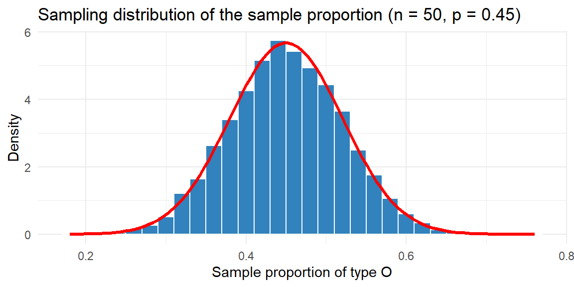
The histogram of the simulated proportions (blue bars) lines up closely with the red Normal curve predicted by the theory. Most sample proportions fall within roughly two standard errors (about ±0.14) of the true proportion 0.45.

Conditions for the normal approximation

The Normal approximation to the sampling distribution of the sample proportion \(\hat{p}\) is extremely useful, but it does not always work well. A common rule of thumb is that both

\[ np \ge 15 \quad \text{and} \quad n(1-p) \ge 15. \]

Here:

\(np\) is the expected number of successes in the sample,
\(n(1-p)\) is the expected number of failures.

The sampling distribution of \(\hat{p}\) is based on the binomial model. When the sample size is small or when the true proportion \(p\) is very close to 0 or 1, the binomial distribution is skewed, not symmetric. In such cases, the bell-shaped Normal curve is a poor approximation.

The conditions \(np \ge 15\) and \(n(1-p) \ge 15\) ensure that:

the distribution of the number of successes is reasonably symmetric,
and there are enough observations in both categories,

When these conditions hold, the sampling distribution of \(\hat{p}\) is well-approximated by a Normal distribution.

If either expected count is too small, several problems arise:

The sampling distribution becomes skewed, often strongly.
The Normal approximation may give inaccurate probabilities.

For example, if a company studies a rare event (say \(p=0.01\)) with only \(n=50\) customers, then

\[ np = 0.5, \]

which is far below 15. The distribution of \(\hat{p}\) in this case is highly right-skewed, and the Normal model performs poorly.

What to do when the condition is not met

When either \(np < 15\) or \(n(1-p) < 15\), it is safer to use methods that do not rely on the Normal approximation, such as:

Exact binomial calculations, which use the true discrete distribution, or
Bootstrap methods (Section 8.4), which approximate the sampling distribution through resampling.

These approaches better capture skewness and discreteness when sample sizes are small or when proportions are extreme.

The Normal approximation for \(\hat{p}\) works well only when there are enough expected successes and failures. Always check the conditions before applying Normal-based inference. When in doubt, especially with small samples or rare events, prefer exact or bootstrap methods to avoid misleading conclusions.

Working in JMP

To explore sampling distributions for proportions in JMP:

Use Analyze → Distribution on a binary variable (coded 1 for success and 0 for failure) to see the data distribution.
Use Graph Builder with the Bootstrap option to resample your data with replacement. Specify the statistic as proportion of successes and the number of bootstrap samples. JMP will display the bootstrap distribution, which closely approximates the theoretical sampling distribution when the sample is random and unbiased.

Recap

Keyword	Definition
Population proportion \(p\)	The true fraction of individuals in the population with a certain characteristic.
Sample proportion \(\hat{p}\)	The fraction of sampled individuals with the characteristic; an estimator of \(p\).
Expected value of \(\hat{p}\)	The expected value of the sampling distribution of \(\hat{p}\), equal to \(p\).
Standard deviation of \(\hat{p}\)	The standard deviation of the sampling distribution of \(\hat{p}\), equal to \(\sqrt{p(1-p)/n}\).
Normal approximation	For large \(n\) with \(np\ge15\) and \(n(1-p)\ge15\), the sampling distribution of \(\hat{p}\) is approximately normal.

Check your understanding

Problems

Explain why the sampling distribution of \(\hat{p}\) has mean equal to the population proportion. What would it mean if the mean of \(\hat{p}\) were systematically above or below \(p\)?
Suppose the true prevalence of a rare mutation is 1%. If you sample \(n=100\) individuals, will the sampling distribution of \(\hat{p}\) be well approximated by a Normal distribution? Why or why not? How might you proceed instead?

Solutions

Unbiasedness. If we took infinitely many random samples and averaged the sample proportions, we would recover the true population proportion. That is precisely what the expected value of \(\hat{p}\) tells us: \(E(\hat{p})=p\). If the mean of \(\hat{p}\) were consistently above \(p\), our estimator would be biased, systematically overestimating the true proportion.
Rare mutation. When \(p\) is very small (0.01) and \(n=100\), the expected number of successes is \(np=1\) and the expected number of failures is 99. Because \(np<15\), the sampling distribution of \(\hat{p}\) is highly skewed and the normal approximation is poor. A better approach is to use the exact binomial distribution to compute probabilities or to use a bootstrap to approximate the sampling distribution (see Section 8.4).

8.3 Sampling Distribution of the Sample Mean

“The Scientist must set in order. Science is built up with facts, as a house is with stones. But a collection of facts is no more a science than a heap of stones is a house.” - Henri Poincare

The sample mean \(\bar{x}\) is the workhorse of quantitative inference. Whenever we measure a quantitative trait—such as revenue per customer, delivery time, exam score, or daily sales—we often reduce the data to a single summary: the average. This simple statistic captures the central tendency of the sample and serves as our primary estimate of the unknown population mean \(\mu\).

But for inference, computing \(\bar{x}\) once is not enough. To draw conclusions about the population, we must understand how \(\bar{x}\) behaves across repeated samples. In other words, we must study the sampling distribution of the sample mean.

Because samples are random, the value of \(\bar{x}\) will vary from sample to sample. If we repeatedly:

Draw a random sample of size \(n\),
Compute the sample mean each time,
Plot all those means,

the resulting distribution is the sampling distribution of \(\bar{x}\).

This distribution tells us:

how close \(\bar{x}\) tends to be to \(\mu\),
how much sampling variability to expect,
and how precise our estimate is likely to be.

These ideas are the foundation of confidence intervals, hypothesis tests, and many statistical models.

Properties of the sampling distribution

Under mild and widely satisfied conditions, the sampling distribution of \(\bar{x}\) has three powerful properties. The first two concern the mean and standard deviation of \(\bar{x}\).

1. The mean of \(\bar{x}\) equals the population mean

If the population has mean \(\mu\), then

\[ E(\bar{x}) = \mu. \]

2. The variability of \(\bar{x}\) shrinks with sample size

The standard deviation of the sampling distribution of \(\bar{x}\) is

\[ \sigma_{\bar{x}} = \frac{\sigma}{\sqrt{n}}, \]

where \(\sigma\) is the population standard deviation.

This quantity is called the standard error of the mean. It shows a crucial fact:

Larger samples produce more precise estimates.

Because of the \(\sqrt{n}\) in the denominator, the variability of \(\bar{x}\) decreases as sample size increases—but with diminishing returns. Doubling the sample size does not cut the error in half; it reduces it by a factor of \(\sqrt{2}\).

The Central Limit Theorem

The third property involves the shape of the sampling distribution of \(\bar{x}\). The Central Limit Theorem (CLT) is one of the pillars of statistics. It states that when we randomly sample from any population with mean \(\mu\) and standard deviation \(\sigma\), the sampling distribution of \(\bar{x}\) becomes approximately normal as the sample size \(n\) grows. In symbols, \[ \bar{X} \overset{\cdot}{\sim} N\bigl(\mu,\, \sigma/\sqrt{n}\bigr) \] for sufficiently large \(n\). Note that the dot (\(\cdot\)) above \(\sim\) means “approximately distributed as”.

The beauty of the CLT is that it does not require the underlying population to be normal; even strongly skewed or irregular distributions yield approximately normal sample means when \(n\) is large enough.

Example 8.4: Simulated Enzyme Activities

Enzyme activity measurements often follow a skewed distribution because they cannot be negative but can have long right tails. Suppose the true activity in a population of cells follows an exponential distribution. We take repeated random samples of different sizes and compute the sample mean for each. The following plot shows 10,000 simulated sample means for \(n=5\), \(n=20\) and \(n=50\) to illustrate how the distribution of \(\bar{x}\) evolves:

The three panels show that for very small samples (\(n=5\)) the sampling distribution of \(\bar{x}\) still retains some skewness. For moderate samples (\(n=20\)) the distribution looks more bell‑shaped, and by \(n=50\) it is nearly indistinguishable from the Normal curve (red line). This behavior is exactly what the CLT predicts.

Practical considerations

The CLT justifies using normal‑based methods for many statistics, but it is not a panacea. Large samples are not always attainable. Sometimes cost, difficulty or the preciousness of biological material limits the sample size. In such cases the sampling distribution of \(\bar{x}\) may be far from normal, especially for very skewed or heavy‑tailed populations. Diagnostic plots and simulation can help you gauge whether normal approximations are reasonable.

If the data is not available, then the rule-of-thumb of \(n\ge 30\) is adequate in most situations to determine if the sample size is large enough.

Working in JMP

To explore the sampling distribution of the mean in JMP:

Use Analyze → Distribution to visualise your quantitative data and estimate the population standard deviation.
Choose Analyze → Resampling and select Bootstrap. Specify the statistic as the mean and set the number of resamples. JMP will generate a bootstrap sampling distribution of \(\bar{x}\), plot it and report the standard error. You can compare the bootstrap distribution to a Normal distribution with mean equal to the observed \(\bar{x}\) and standard deviation equal to the bootstrap standard error.

Recap

Keyword	Definition
Standard deviation of \(\bar{x}\)	The standard deviation of the sampling distribution of \(\bar{x}\), equal to \(\sigma/\sqrt{n}\).
Central Limit Theorem (CLT)	States that for large \(n\), the sampling distribution of the sample mean is approximately normal with mean \(\mu\) and standard deviation \(\sigma/\sqrt{n}\).

Check your understanding

Problems

A laboratory measures the enzyme activity of 10 randomly selected yeast cultures. The population distribution is known to be highly skewed with mean 50 units and standard deviation 20 units. Without doing any calculations, would you expect the sample mean to follow a Normal distribution? Explain your reasoning.
A nutritionist samples 64 adults and measures their daily vitamin D intake. The population mean intake is 600 IU with standard deviation 200 IU. What is the mean and standard deviation of the sampling distribution of \(\bar{x}\)? If the intake distribution is skewed, is the Normal approximation still reasonable? Why or why not?

Solutions

Small, skewed samples. With a sample size of 10 and a highly skewed population, the sampling distribution of \(\bar{x}\) will retain noticeable skewness. The Central Limit Theorem requires larger \(n\) before the distribution of the sample mean becomes approximately normal, so caution is warranted when applying Normal approximations.
Vitamin D intake. The sampling distribution has mean \(\mu = 600\) and standard deviation \(200/\sqrt{64} = 25\). Because \(n=64\) is reasonably large, the CLT suggests that the sample mean will be approximately normal even if the individual intakes are skewed. Therefore the Normal approximation should be adequate.

8.4 Bootstrap Sampling Distribution

“It is the mark of a truly intelligent person to be moved by statistics.” -George Bernard Shaw

Sometimes we cannot rely on tidy formulas or the Central Limit Theorem (CLT) to determine the sampling distribution of a statistic. The CLT works beautifully for sample means under broad conditions, but many practical situations fall outside its comfort zone. For example:

The statistic of interest may have a complicated distribution (such as the median, a trimmed mean, a percentile, or a regression coefficient).
The sample size may be too small for Normal approximations to be reliable.
The population distribution may be strongly skewed or heavy-tailed.
The standard error formula may be unknown or difficult to derive.

In these settings, classical theoretical methods either become inaccurate or require mathematics that is impractical to work out by hand. Bootstrapping provides a powerful, data-driven alternative.

Bootstrapping is a resampling method that approximates the sampling distribution of a statistic by using the data we already have. Instead of imagining all possible samples from the population (which we cannot see), we treat the observed sample as a stand-in for the population and repeatedly resample from it.

The name comes from the phrase “pulling yourself up by your bootstraps”—we use the sample to learn about its own variability.

The key insight is:

If the sample is representative of the population, then resampling from the sample mimics sampling from the population.

How bootstrapping works

Suppose we have a sample of size \(n\) and a statistic of interest (say the median).

A bootstrap procedure typically follows these steps:

Start with the original sample of size \(n\).
Resample with replacement from the sample to create a bootstrap sample of size \(n\).
Compute the statistic (e.g., the median) for this bootstrap sample.
Repeat steps 2–3 many times (often thousands).
Examine the distribution of the bootstrap statistics.

The resulting distribution is called the bootstrap distribution, and it serves as an approximation to the true sampling distribution of the statistic.

Example 8.5: Median Tumor Size

Imagine a study measuring the diameters (in millimeters) of 25 tumors detected in a mammogram screening. The sample is small and the data are skewed; we want to estimate the sampling distribution of the median tumor size. A bootstrap approach provides the following:

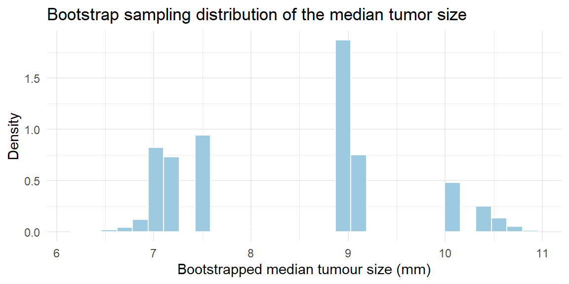
The histogram shows the bootstrap distribution of the median tumor size. From this distribution we can compute a bootstrap standard deviation (the standard deviation of the bootstrap medians) and make inferences.

Why bootstrapping is useful

Bootstrapping is especially valuable when:

the sampling distribution is mathematically intractable,
the statistic is not well handled by the CLT,
the sample size is modest,
or we want a flexible, computer-based solution.

From the bootstrap distribution we can estimate:

the standard error of the statistic,
confidence intervals,
bias in the estimator,
and the overall shape of the sampling distribution.

In modern statistics, bootstrapping is widely used because it replaces difficult mathematics with computation.

When to be cautious

Bootstrapping is powerful but not magic. It works best when:

the original sample is representative of the population,
observations are independent,
and the sample size is not extremely small.

If the sample is biased or too tiny to reflect the population’s structure, the bootstrap will faithfully reproduce those problems.

The big picture

Classical inference relies on theoretical sampling distributions derived from probability models. Bootstrapping takes a different approach:

Theory-based inference: derive the sampling distribution mathematically.
Bootstrap inference: approximate the sampling distribution computationally.

When formulas are unavailable or unreliable, bootstrapping provides a practical and remarkably effective way to understand the variability of complex statistics directly from the data.

Working in JMP

JMP has built‑in bootstrap tools that make resampling easy:

After running an analysis (for example Analyze → Fit Y by X for comparing two groups), click the red triangle menu (▸) and select Bootstrap. Choose the statistic you wish to bootstrap and the number of resamples. JMP will create a bootstrap distribution, display it and report standard errors and confidence intervals.
For custom statistics, use Tables → Bootstrap Data to generate bootstrap samples from your dataset. You can then analyse each bootstrap sample using your preferred platform and collect the statistic of interest.

Recap

Keyword	Definition
Bootstrapping	A resampling method that uses the observed data to approximate a sampling distribution by repeatedly sampling with replacement.
Bootstrap sample	A sample of size \(n\) drawn with replacement from the original sample.
Bootstrap statistic	The value of the statistic computed on a bootstrap sample.
Bootstrap distribution	The distribution of many bootstrap statistics; an empirical approximation to the sampling distribution.

Check your understanding

Problems

Why do we sample with replacement when constructing a bootstrap sample? What would go wrong if we sampled without replacement?
Compare and contrast the bootstrap distribution with the theoretical sampling distribution. Under what circumstances do they coincide, and when might they differ?

Solutions

Replacement is essential. Sampling with replacement allows each observation to appear multiple times—or not at all—in a bootstrap sample. This mimics the variability of drawing new samples from the population. Sampling without replacement would simply rearrange the data and fail to capture the variability inherent in new samples.
Bootstrap vs. theoretical. The bootstrap distribution approximates the theoretical sampling distribution when the sample is random and representative, and when the number of bootstrap resamples is large. For statistics with simple known sampling distributions (like means and proportions), the bootstrap will agree closely with theory. For statistics whose sampling distributions are complicated or unknown, the bootstrap provides a practical alternative but may differ from the true sampling distribution, especially when the sample size is very small or the sample is biased.

Data was obtained from Introductory Statistical Methods classes. Here, we are treating these values as a population.↩︎