5  Week 2: Random Variables

5.1 Why This Matters

Last section, we worked with probabilities of events (a transaction is fraudulent, a call converts, a unit is defective). To go further to compute an expected profit, describe how a count of monthly defects varies, or eventually build the probability distributions behind confidence intervals, we need a way to attach a number to an uncertain outcome and describe how likely each possible number is. That’s what a random variable does, and it’s the building block for everything else in this module.

5.2 What Is a Random Variable?

A random variable is a rule that assigns a numerical value to each outcome of a random process. Formally, it’s a function whose domain is the sample space and whose range is a set of numbers, but informally, it’s just the “number we care about” from an uncertain situation.

ExampleExample 2.11: Turning outcomes into numbers

An online retailer wants to study how many items customers add to their cart during a single visit. The underlying outcome (a customer’s entire browsing session) is complicated: pages viewed, time spent, items considered and rejected. The random variable \[ X = \text{number of items added to the cart} \] distills all of that complexity down to a single number. Before we observe a given customer’s session, \(X\) could be 0, 1, 2, 3, or more. Once the session ends, we observe one specific value—say \(x=2\), which is called a realization of \(X\).

Random variables come in two broad types:

  • A discrete random variable takes a countable set of values, usually arising from counting: number of items in a cart, number of support tickets filed today, number of defective units in a shipment.
  • A continuous random variable can take any value in an interval: the time until a support ticket is resolved, the exact weight of a shipped package. We’ll study continuous random variables in an upcoming week; for now, our focus is discrete random variables.
NoteA random variable describes a process, not a single dataset

Before a call center’s shift starts, “number of complaints received today” is unknown and could take many values - that’s the random variable. Once the shift ends and we’ve counted 7 complaints, that 7 is one realization, not the random variable itself. Run the same shift again next week and you’ll likely observe a different number, even though nothing about the underlying process changed. This is why we use an uppercase letter (\(X\)) for the random variable and a lowercase letter (\(x\)) for an observed realization.

5.3 Probability Distributions

Once we have a discrete random variable, the next step is describing how likely each of its possible values is. A probability distribution assigns a probability \(P(X=x)\) to every possible value \(x\). Any valid probability distribution must satisfy two conditions:

  1. Non-negativity: every probability satisfies \(0 \le P(X=x) \le 1\).
  2. Sums to one: \(\displaystyle\sum_x P(X=x) = 1\), something in the sample space has to happen.
ExampleExample 2.12: Distribution of items per cart

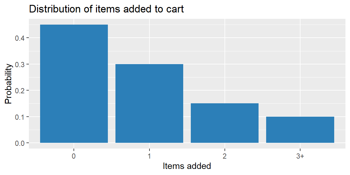
Based on a large sample of past sessions, the retailer estimates the following distribution for \(X\) = number of items added to the cart:

\(x\) 0 1 2 3 or more
\(P(X=x)\) 0.45 0.30 0.15 0.10

Every probability is between 0 and 1, and they sum to \(0.45+0.30+0.15+0.10=1\), so this is a valid distribution. It tells the retailer that, over many sessions, about 45% end with an empty cart, 30% with exactly one item, and so on.

library(tidyverse)

cart_dist <- tibble(
  items = c("0", "1", "2", "3+"),
  prob  = c(0.45, 0.30, 0.15, 0.10)
)

ggplot(cart_dist, aes(x = items, y = prob)) +
  geom_col(fill = "#2c7fb8") +
  labs(title = "Distribution of items added to cart", x = "Items added", y = "Probability")

NoteChecking whether a proposed distribution is valid

Given a proposed distribution, check both conditions before using it: are all the probabilities between 0 and 1, and do they sum to 1 (allowing for small rounding)? A distribution that fails either check (e.g., includes a negative probability, or sums to 1.1) cannot be a real probability distribution and needs to be corrected first.

5.4 Expected Value and Variance of a Random Variable

Just as we describe a sample with statistics like \(\bar{x}\) and \(s\), we describe a random variable (really, an entire population or process) with parameters, typically written with Greek letters (\(\mu\), \(\sigma\), \(\sigma^2\)).

Expected Value

The expected value (or mean) of a discrete random variable is a probability-weighted average of its possible values: \[ \mu = E(X) = \sum_x x \cdot P(X=x) \] You can think of \(E(X)\) as the long-run average of \(X\) if the underlying process were repeated many, many times—it is not necessarily a value \(X\) can actually take on any single trial.

ExampleExample 2.13: Should we sell an extended warranty?

An electronics retailer sells a $1,200 laptop and is deciding whether to offer a one-year extended warranty for $80. Based on historical claims data, there’s a 6% chance a customer will file a claim during that year, and the average repair cost on a valid claim is $650. Let \(X\) = profit to the retailer per warranty sold:

  • If no claim is filed: profit is \(\$80\).
  • If a claim is filed: profit is \(\$80 - \$650 = -\$570\).

\[ \begin{align*} E(X) &= (80)(0.94) + (-570)(0.06)\\ &= 75.20 - 34.20\\ &= 41.00 \end{align*} \]

On average, the retailer expects to make $41 per warranty sold, even though any individual warranty either nets $80 (no claim) or loses $570 (a claim). This is exactly why insurance and warranty products are priced this way: the expected value is positive for the seller even though any single outcome could be a loss.

NoteExpected value is a long-run average, not a prediction

\(E(X) = \$41\) does not mean the retailer makes $41 on every warranty—no single customer’s outcome will actually equal $41. It means that if the retailer sells this warranty to thousands of similar customers, the average profit per warranty will be close to $41. Expected value is a planning tool for volume, not a forecast for one transaction.

ExampleExample 2.14: The Florida Lottery

Expected value doesn’t have to come out positive, it’s just as useful for showing when a “bet” is a bad one, on average. The Florida Lottery runs two popular daily games, Pick 3 and Pick 4.

In Pick 3, players pay $1 to select three numbers in order, each ranging from 0 to 9. If all three numbers match the order of the numbers drawn, the player wins $500. The probability of winning Pick 3 is 0.001.

Let \(X\) be the amount of money a player nets from a single Pick 3 ticket. The possible values are:

  • If the player loses: \(X = -\$1\)
  • If the player wins: \(X = \$500 - \$1 = \$499\)

\[ \begin{align*} E(X) &= (-1)(0.999) + (499)(0.001)\\ &= -0.999 + 0.499\\ &= -0.50 \end{align*} \]

Pick 4 is similar, but players must match four numbers in order for a $5,000 payout, and the probability of winning is only 0.0001. Let \(X\) be the net amount from a single Pick 4 ticket:

  • If the player loses: \(X = -\$1\)
  • If the player wins: \(X = \$5{,}000 - \$1 = \$4{,}999\)

\[ \begin{align*} E(X) &= (-1)(0.9999) + (4999)(0.0001)\\ &= -0.9999 + 0.4999\\ &= -0.50 \end{align*} \]

Both games have the same expected value: -$0.50 per ticket. Despite very different odds and payouts, a player loses 50 cents on average for every dollar wagered, on either game. This is exactly how lottery games (and casinos) are designed to work: the expected value to the player is reliably negative, which is what makes the expected value to the operator reliably positive, the same logic as the warranty example above, just from the other side of the transaction.
Variance and Standard Deviation

The variance of \(X\) measures how spread out its values are around the mean: \[ \sigma^2 = \sum_x (x-\mu)^2 \cdot P(X=x) \] The standard deviation, \(\sigma = \sqrt{\sigma^2}\), is in the same units as \(X\) and describes a typical distance from the mean.

ExampleExample 2.15: Variability in items returned per order

A retailer’s data shows the number of items returned per order, \(Y\), follows this distribution:

\(y\) 0 1 2 3
\(P(Y=y)\) 0.70 0.20 0.07 0.03

The expected number of items returned per order is \[ \mu_Y = 0(0.70) + 1(0.20) + 2(0.07) + 3(0.03) = 0.43 \]

To find the variance, compute \((y-\mu)^2\) for each value, weight by its probability, and sum:

\(y\) \((y - 0.43)^2\) \(P(Y=y)\) Contribution
0 0.1849 0.70 0.12943
1 0.3249 0.20 0.06498
2 2.4649 0.07 0.17254
3 6.6049 0.03 0.19815

\[ \sigma_Y^2 = 0.12943 + 0.06498 + 0.17254 + 0.19815 \approx 0.5651 \] \[ \sigma_Y = \sqrt{0.5651} \approx 0.752 \]

An average order has 0.43 returned items, with a typical order deviating from that average by about 0.75 items. Note that neither the mean nor the standard deviation has to equal a value \(Y\) can actually take, you cannot return 0.43 items, they summarize the distribution, not any one order.

ExampleExample 2.16: Computing expected value and variance in R
returns <- tibble(
  y = c(0, 1, 2, 3),
  prob = c(0.70, 0.20, 0.07, 0.03)
)

mu <- sum(returns$y * returns$prob)
var <- sum((returns$y - mu)^2 * returns$prob)

mu
[1] 0.43
var
[1] 0.5651
sqrt(var)
[1] 0.7517313

In Excel, the same calculation uses SUMPRODUCT(): =SUMPRODUCT(y_range, prob_range) for the mean, and a helper column for \((y-\mu)^2\) multiplied into SUMPRODUCT() again for the variance.

5.5 Recap

Keyword Definition
Random variable A rule that assigns a numerical value to each outcome of a random process.
Discrete random variable A random variable with a countable set of possible values (e.g., a count).
Continuous random variable A random variable that can take any value within an interval (e.g., a measurement).
Realization The specific observed value of a random variable after the process occurs.
Probability distribution An assignment of probabilities to every possible value of a random variable; must be non-negative and sum to 1.
Expected value \(E(X) = \sum_x x\,P(X=x)\); the probability-weighted long-run average of \(X\).
Variance / standard deviation \(\sigma^2 = \sum_x (x-\mu)^2 P(X=x)\); measures how spread out \(X\)’s values are around its mean.

5.6 Check Your Understanding

NoteProblems
  1. A ride-share company defines \(X\) = number of cancellations per driver shift. Is \(X\) discrete or continuous? What are some plausible values it could take?

  2. A proposed distribution for the number of defective units in a shipment of 4 items is: \(P(X=0)=0.6\), \(P(X=1)=0.25\), \(P(X=2)=0.1\), \(P(X=3)=0.1\), \(P(X=4)=0\). Is this a valid probability distribution? If not, explain why.

  3. A subscription box company charges $30/month and estimates that 5% of customers will cancel and request a full refund each month, while the rest keep the box (no refund). Let \(X\) = revenue per customer per month. Compute \(E(X)\).

  4. Using the distribution from Problem 3, would you expect every individual customer to generate close to \(E(X)\) in a given month? Why or why not?

  1. \(X\) is discrete—cancellations are counted, not measured. Plausible values are \(0, 1, 2, 3, \dots\) up to however many rides a driver could plausibly be assigned in a shift.

  2. Not valid. The probabilities sum to \(0.6+0.25+0.1+0.1+0=1.05\), which exceeds 1, so this cannot be a real probability distribution (even though each individual value is between 0 and 1).

  3. Let \(X\) = revenue per customer. If the customer cancels: \(X = \$0\) (full refund). If not: \(X = \$30\). \[ E(X) = (30)(0.95) + (0)(0.05) = 28.50 \] Expected monthly revenue per customer is $28.50.

  4. No. Every individual customer generates either exactly $0 or exactly $30—no one actually pays $28.50. The expected value is a long-run average across many customers, useful for forecasting total revenue across the subscriber base, not for predicting any one customer’s outcome.