7 Week 3: The Uniform Distribution

7.1 Why This Matters

The binomial distribution counts things, a whole number of successes out of a fixed number of trials. Many business quantities aren’t counts at all: a delivery time, a wait time, a dollar amount. These are continuous random variables, which can take any value within a range rather than a countable list of values. We’ll spend the next two sections on continuous distributions, starting with the simplest one, the uniform distribution, before moving to the single most important one, the normal distribution. The uniform distribution isn’t just a warm-up exercise, either. It’s the engine behind every random number your computer generates, which makes it the natural starting point for simulation, something we’ll lean on again later in this course.

7.2 From Discrete to Continuous

A continuous random variable can take any value in an interval: a delivery could arrive at 2:00pm, 2:01pm, or 2:00:47.3pm. Because there are infinitely many possible values, it doesn’t make sense to ask for the probability of one exact value, that probability is always 0. Instead, we ask for the probability that the variable falls in some range, and we get that probability from the area under a curve describing the distribution, rather than from a table like we used for discrete random variables.

For most continuous distributions, computing that area requires calculus. The uniform distribution is the happy exception: its curve is just a flat rectangle, so the area is nothing more than base times height arithmetic, not calculus.

7.3 The Uniform Distribution

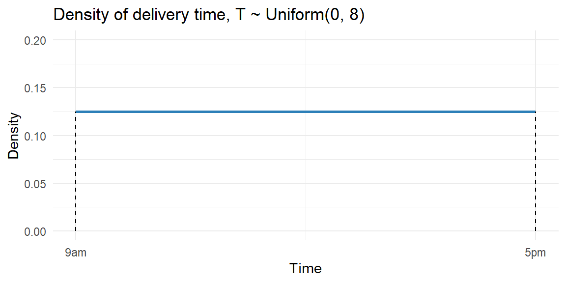
A continuous random variable \(X\) follows a Uniform\((c,d)\) distribution if every value between \(c\) and \(d\) is equally likely, and no value outside that range is possible. Its density is a flat, horizontal line of height \(\dfrac{1}{d-c}\) across the interval \((c,d)\)—a rectangle, chosen so that its total area equals 1 (as it must, since total probability is always 1).

Example 3.6: A same-day delivery window

A retailer promises same-day delivery “sometime between 9am and 5pm,” and internally, the delivery time is equally likely to be any moment in that 8-hour window. Let \(T\) = hours after 9am that the delivery arrives, so \(T \sim \text{Uniform}(0, 8)\).

Because the density is a flat rectangle, the probability that \(X\) falls between any two points \(a\) and \(b\) (with \(c \le a < b \le d\)) is simply the width of that interval divided by the total width: \[ P(a < X < b) = \frac{b-a}{d-c} \]

Example 3.7: Probability of a noon-to-1pm delivery

Continuing Example 3.6, what’s the probability a delivery arrives between noon and 1pm? Noon is 3 hours after 9am and 1pm is 4 hours after 9am, so \(a=3\), \(b=4\), and the full window is \((c,d)=(0,8)\): \[ P(3 < T < 4) = \frac{4-3}{8-0} = \frac{1}{8} = 0.125 \] Notice that this only depends on the length of the target interval (1 hour) relative to the length of the whole window (8 hours)—not on where in the window it falls. A 1-hour window from 2pm to 3pm would give exactly the same probability.

The mean and standard deviation of a Uniform\((c,d)\) distribution have simple closed forms: \[ \mu = \frac{c+d}{2} \qquad\qquad \sigma = \frac{d-c}{\sqrt{12}} \]

Example 3.8: Mean and SD of the delivery window

For \(T \sim \text{Uniform}(0,8)\) from Example 3.6: \[ \begin{align*} \mu &= \frac{0+8}{2} = 4 \text{ hours after 9am (i.e., 1pm)}\\\\ \sigma &= \frac{8-0}{\sqrt{12}} \approx 2.31 \text{ hours} \end{align*} \] The “expected” delivery time is 1pm, right in the middle of the window, which makes sense given every moment in the window is equally likely.

7.4 The Uniform Distribution and Simulation

Here’s why the uniform distribution matters beyond describing delivery windows: it’s the building block behind essentially every random simulation you’ll run in this course. When Excel’s RAND() or R’s runif() generates a “random number,” it’s drawing from a Uniform(0,1) distribution—and every other kind of randomness a computer simulates (random assignment to a treatment group, a Monte Carlo scenario, a shuffled sample) is built by transforming draws from that same Uniform(0,1) starting point.

Example 3.9: Uniform probabilities and simulation in R and Excel

To compute the exact probability from Example 3.7 in R, use punif():

punif(4, min = 0, max = 8) - punif(3, min = 0, max = 8)

[1] 0.125

This matches our by-hand answer of 0.125: it’s the cumulative probability up to 4 hours, minus the cumulative probability up to 3 hours.

To simulate 10,000 random delivery times and check that they behave the way theory predicts:

library(tidyverse)

set.seed(2025)
sim_deliveries <- runif(10000, min = 0, max = 8)
mean(sim_deliveries)                              # should be close to 4

[1] 3.994016

mean(sim_deliveries > 3 & sim_deliveries < 4)      # should be close to 0.125

[1] 0.123

In Excel, =RAND()*8 generates a single simulated delivery time on \((0,8)\), and dragging that formula down a column simulates many deliveries at once—the same logic we’ll use later in the course to build simulation-based what-if analyses.

7.5 Recap

Keyword	Definition
Continuous random variable	A random variable that can take any value within an interval; the probability of any single exact value is 0.
Uniform distribution	A continuous distribution on \((c,d)\) where every value in the interval is equally likely; density is constant at \(1/(d-c)\).
Uniform probability rule	\(P(a<X<b) = (b-a)/(d-c)\)—the ratio of interval lengths.
Uniform mean and SD	\(\mu = (c+d)/2\), \(\sigma = (d-c)/\sqrt{12}\).

7.6 Check Your Understanding

Problems

A ride-share app tells riders their driver will arrive “in 2 to 10 minutes,” and arrival time within that window is equally likely at any point. Let \(X\) = arrival time in minutes. What distribution does \(X\) follow, and what are its mean and standard deviation?
Using the distribution from Problem 1, what is the probability the driver arrives within the first 4 minutes (between 2 and 4 minutes)?
A factory’s automated filling machine dispenses between 495 mL and 505 mL into a bottle, uniformly at random. What’s the probability a randomly selected bottle contains between 498 and 502 mL?
Explain, without doing any calculation, why \(P(2 < X < 3)\) and \(P(7 < X < 8)\) are equal for the ride-share example in Problem 1.

Solutions

\(X \sim \text{Uniform}(2, 10)\). \(\mu = (2+10)/2 = 6\) minutes. \(\sigma = (10-2)/\sqrt{12} \approx 2.31\) minutes.
\(P(2 < X < 4) = \dfrac{4-2}{10-2} = \dfrac{2}{8} = 0.25\).
Let \(Y \sim \text{Uniform}(495, 505)\). \(P(498 < Y < 502) = \dfrac{502-498}{505-495} = \dfrac{4}{10} = 0.4\).
For a uniform distribution, the probability of an interval depends only on the interval’s length, not its location within \((c,d)\). Both \((2,3)\) and \((7,8)\) have length 1, and both lie within the Uniform\((2,10)\) range, so they have the same probability regardless of where they fall in the window.