5 Probability Concepts

5.1 Basic Probability Rules

“The theory of probabilities is at bottom nothing but common sense reduced to calculus.” – Pierre‑Simon Laplace

When people say “there’s a 70 percent chance of rain” or that a team has “even odds” of winning, they’re using probability to express how likely an outcome seems. In statistics, we give that vague notion a precise meaning. A probability is a number between 0 and 1 that measures how often we expect an event to occur in the long run.

A probability of 0 means the event can never happen, a probability of 1 means it is certain, and values in between describe varying degrees of likelihood.

Experiments, outcomes and sample spaces

Probability always starts with an experiment—a repeatable situation whose result is not predetermined.

Flipping a coin, rolling a die or drawing a card are familiar examples. Each trial produces an outcome, and the set of all possible outcomes is called the sample space.

We often use \(S\) to denote the sample space. For instance, when you flip one fair coin, the sample space is \(S=\{\text{H},\text{T}\}\); when you roll a six‑sided die, \(S=\{1,2,3,4,5,6\}\).

It is essential to describe the sample space clearly because the probability of any event is computed relative to it. In practice, the sample space can be finite (like the faces of a die) or infinite (like all possible real‑valued measurements of temperature). Identifying \(S\) helps us keep track of what outcomes are possible before we assign probabilities.

Events and interpretations of probability

An event is any subset of the sample space. Events can be simple (containing one outcome) or compound (containing several outcomes).

Let \(A\) be the event that a die roll is even. Then \(A=\{2,4,6\}\), which contains three outcomes from the sample space \(S=\{1,2,3,4,5,6\}\).

The probability of an event \(A\), written \(P(A)\), quantifies how likely \(A\) is to occur.

When the outcomes in \(S\) are equally likely (as with a fair die or fair coin), the classical probability of \(A\) is

\[ P(A) = \frac{\text{number of outcomes in }A}{\text{number of outcomes in }S}\,. \]

In the die example above, there are three even numbers out of six, so \(P(A)=3/6=0.5\). This agrees with our intuition that even and odd numbers are equally likely on a fair die.

Probability has several interpretations. In the frequentist view, \(P(A)\) is the long‑run relative frequency of \(A\)—the fraction of times \(A\) occurs if we repeat the experiment many times under identical conditions. For example, the probability of flipping a head on a fair coin is 0.5 because, in the long run, about half of the flips will show heads.

Example 5.1: Rolling a six-sided die

Suppose we rolled a six-sided die 20 times. Using the idea of equally likely outcomes, the probability of rolling a six is \[ \begin{align} P(6)=&\frac{1}{6}\\ \approx& 0.167 \end{align} \] Let’s see how many times we get a six when rolling the die 20 times.

3	6	1	5	5	4	3	2	2	6	1	2	3	3	1	1	3	5	3	2

We see that we rolled a six 2 out of the 20 times. The relative frequency is thus \[ \frac{\text{number of sixes}}{\text{number of rolls}}=\frac{2}{20}=0.1 \]

Let’s look at a bar chart for all of the rolls:

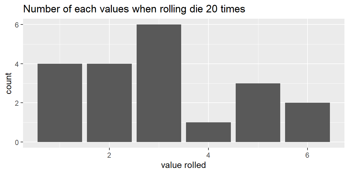
Let’s now roll the die 1,000 times:

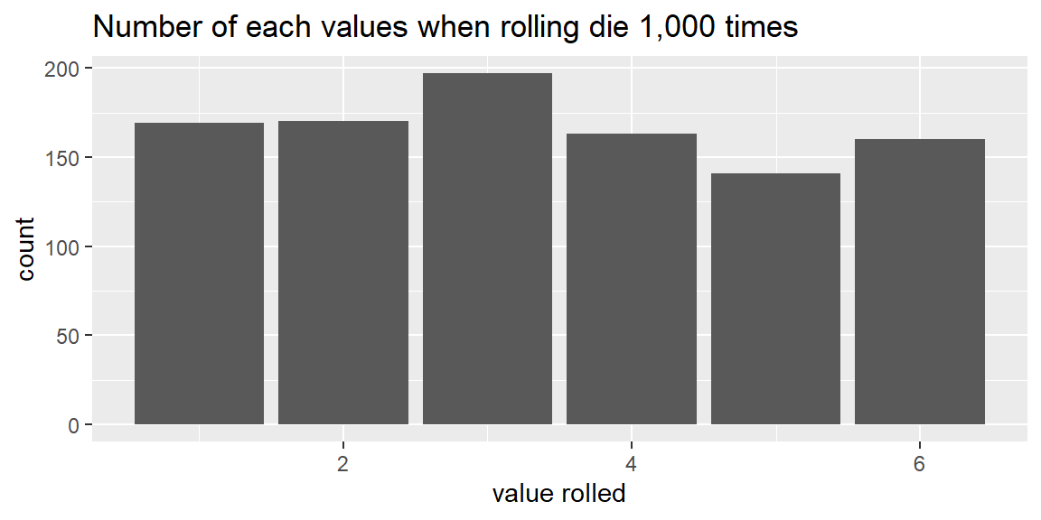
The number of times we rolled each value is a little more even. Focusing only on six, we have \[ \frac{\text{number of sixes}}{\text{number of rolls}}=\frac{160}{1000}=0.16 \] which is close to the theoretical proportion of \(1/6\approx 0.167\)

We can keep increasing the number of times we roll the die and we will see the number of each value “even out” across all values:

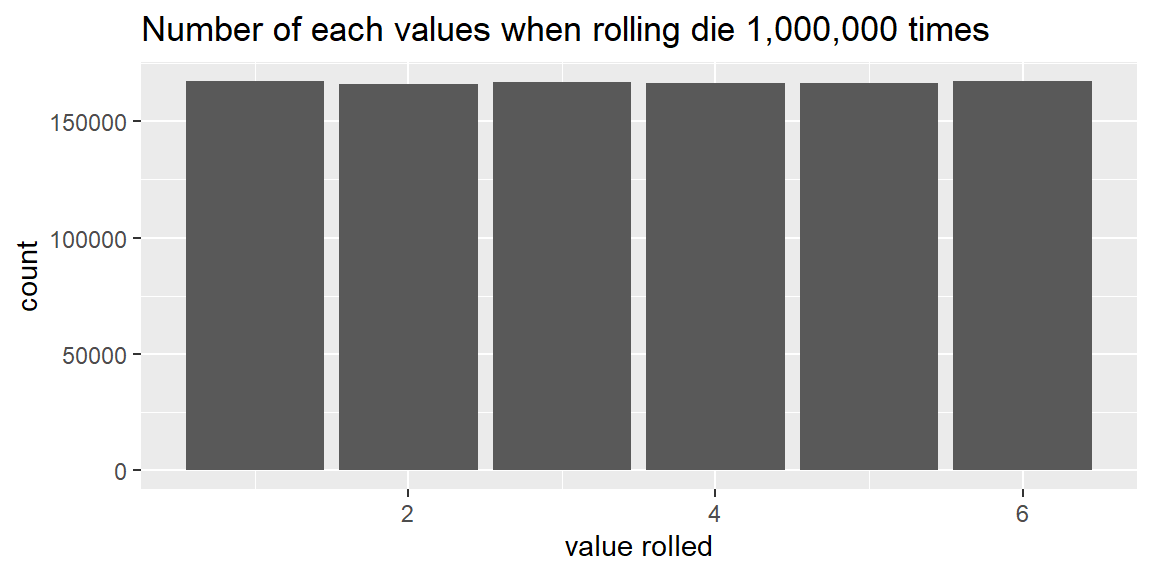
Each value will converge to the theoretical value of \(1/6\).

Example 5.2: Flipping a coin

Suppose we flip a coin many times and track the proportion of heads over time. Early on, the proportion jumps around; as the number of flips grows, it tends to settle near the true probability of 0.5.

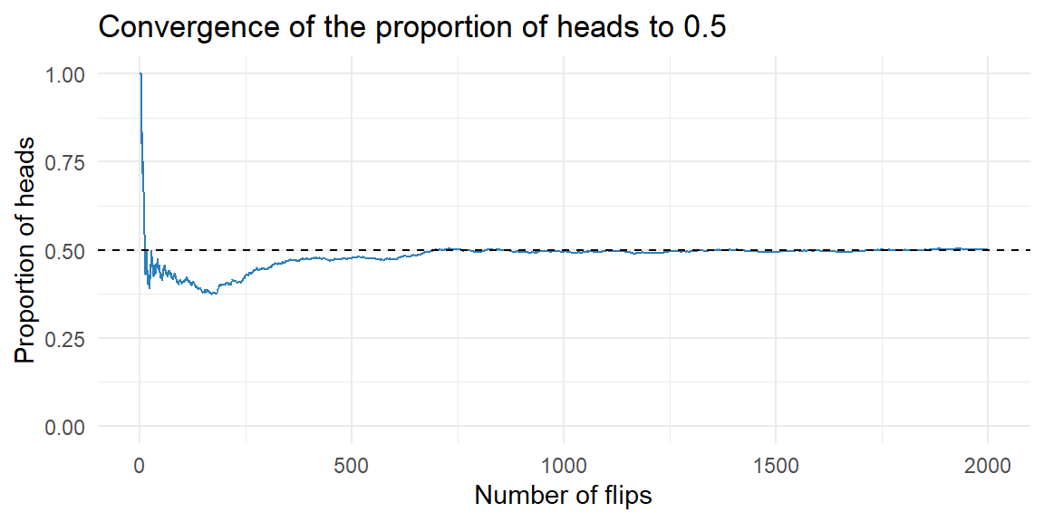
Law of Large Numbers

In 1689, the Swiss mathematician Jacob Bernoulli proved that as the number of trials increases, the proportion of occurrences of any given outcome approaches a particular number (such as 1/6 or 1/2) in the long run.

To show this, he assumed that the outcome of any one trial does not depend on the outcome of any other trial. Bernoulli’s result is known as the Law of Large Numbers.

We will interpret the probability of an outcome to represent long-run results. This is the frequentist approach to probability.

Frequentist and Subjective probability

Probability can be defined in different ways:

Frequentist (long‑run relative frequency). For repeatable experiments, \(P(A)\) is the limit of the proportion of times \(A\) occurs in a large number of trials.
Subjective. Probability reflects a personal belief based on available information; two people may assign different probabilities to the same event.

No matter how you interpret it, probability values lie between 0 and 1 and follow certain algebraic rules.

Complements and the complement rule

If \(A\) is an event, the complement of \(A\) (denoted \(A^c\)) consists of all outcomes in \(S\) that are not in \(A\). In everyday terms, either \(A\) happens or it doesn’t, so the probabilities of \(A\) and its complement must sum to 1. This leads to the complement rule:

\[ P(A^c) = 1 - P(A) \]

The complement rule is especially handy for “at least one” problems. Suppose you toss a fair coin three times and want the probability of getting at least one head. Let \(A\) be the event “at least one head” and \(A^c\) be “no heads” (all tails). There are eight possible equally likely outcomes in the sample space \[ S=\left\{HHH, HHT, HTH, HTT, THH, THT, TTH, TTT\right\} \]

There is only one outcome with no heads—TTT—so \(P(A^c)=1/8\).

By the complement rule, \(P(A)=1-1/8=7/8\).

Unions, intersections and the addition rule

When you combine events, you need to think about unions and intersections. The union of two events \(A\) and \(B\) (written \(A\cup B\)) contains outcomes that are in \(A\) or in \(B\) (or in both).

The intersection of \(A\) and \(B\) (written \(A\cap B\)) contains outcomes that are in both \(A\) and \(B\). The probability of the union is given by the general additive rule:

\[ P(A\cup B) = P(A) + P(B) - P(A\cap B)\,. \]

Example 5.3: Additive rule

Imagine a survey of 200 students about their beverage preferences:

120 students like coffee.
90 students like tea.
60 students like both coffee and tea.

Define event \(C\) = “student likes coffee” and event \(T\) = “student likes tea.” Then

\(P(C) = 120/200 = 0.60\)
\(P(T) = 90/200 = 0.45\)
\(P(C\cap T) = 60/200 = 0.30\)

The probability that a randomly chosen student likes either coffee or tea (or both) is

\[ \begin{align*} P(C\cup T) =& P(C) + P(T) - P(C\cap T)\\ =& 0.60 + 0.45 - 0.30\\ =& 0.75 \end{align*} \]

So 75% of students like at least one of the two beverages.

Notice that this formula counts how many like coffee (\(P(C)\)). Then it adds how many like tea (\(P(T)\)). When these two are added together, the students who like both coffee and tea are added twice: once in \(P(C)\) and again in \(P(T)\). Therefore, those students must be subtracted off one time. That is why we subtract off the intersection \(P(C\cap T)\).

Mutually Exclusive

If \(A\) and \(B\) are mutually exclusive (also called disjoint)—meaning they have no outcomes in common—then \(P(A\cap B)=0\) and the rule simplifies to \(P(A\cup B)=P(A)+P(B)\). A simple example involves rolling a die. Let \(A\) be “rolling a 2” and \(B\) be “rolling an odd number.” These events are disjoint because 2 is even, so \[ P(A\cup B)=P(\text{2})+P(\text{odd})=1/6+3/6=2/3 \]

Example 5.4: Hospital patients

Hospital records show that 12% of all patients are admitted for surgical treatment, 16% are admitted for obstetrics, and 2% receive both obstetrics and surgical treatment.

If a new patient is admitted to the hospital, what is the probability that the patient will be admitted for surgery, for obstetrics, or for both?

Let \(A=\{\text{A patient admitted to the hospital receives surgical treatment.}\}\)
and \(B=\{\text{A patient admitted to the hospital receives obstetrics treatment.}\}\)

We have \[ P(A) = 0.12\qquad P(B) = 0.16\qquad P(A\cap B) = 0.02 \] Since some patients receives both surgical and obstetrics treatments, these events are not mutually exclusive. The general addition rule gives

\[ \begin{align*} P(A\cup B) &= P(A) + P(B) -P(A\cap B) \\ & = 0.12+.016-.02\\ & = 0.26 \end{align*} \]

Thus, 26% of all patients admitted to the hospital receive either surgical treatment, obstetrics treatment, or both.

Probability from contingency tables

Given a contingency table where the data is displayed by two categorical variables, we can estimate the probabilities by using the frequencies in the cells.

Example 5.5: Credit card fraud detection

A bank reviews 10,000 credit card transactions and uses an independent audit to establish whether each one was truly fraudulent. Of the 500 transactions that were actually fraudulent, the bank’s fraud-detection algorithm flagged 400 as suspicious (and missed 100); of the 9,500 legitimate transactions, the algorithm flagged 950 incorrectly (false alarms) and cleared 8,550. Thus 1,350 transactions were flagged, but only 400 of them were genuinely fraudulent.

Fraud status	Algorithm: Flagged	Algorithm: Cleared	Total
Fraud present	400	100	500
Fraud absent	950	8,550	9,500
Total	1,350	8,650	10,000

We can estimate probabilities by dividing each cell count by the total number of transactions (10,000). For example, the probability that a randomly selected transaction is fraudulent is \[ P(\text{Fraud})=\frac{500}{10{,}000}=0.05 \]

The probability that a transaction is fraudulent and flagged by the algorithm is \[ P(\text{Fraud}\cap\text{Flagged})=\frac{400}{10{,}000}=0.04 \]

For a union, we apply the additive rule. The probability that a transaction is fraudulent or flagged (or both) is \[ \begin{align*} P(\text{Fraud}\cup\text{Flagged}) &= P(\text{Fraud})+P(\text{Flagged})-P(\text{Fraud}\cap\text{Flagged})\\ &= \frac{500}{10{,}000}+\frac{1{,}350}{10{,}000}-\frac{400}{10{,}000}\\ &= \frac{1{,}450}{10{,}000}\\ &= 0.145 \end{align*} \]

Recap

Keyword	Definition
Probability	A number between 0 and 1 measuring how likely an event is to occur.
Experiment	A repeatable process with uncertain outcome (e.g., flipping a coin, rolling a die).
Outcome	A single possible result of an experiment; elements of the sample space.
Sample space	The set of all possible outcomes of an experiment.
Event	A subset of the sample space; may include one or many outcomes.
Frequentist interpretation	Defines probability as the long‑run relative frequency of an event in repeated trial.

Check your understanding

Problems

Describe the parts of a probability model. In your own words, explain the difference between an outcome, an event and a sample space. Use the experiment of rolling a six‑sided die as an example.
Equally likely probability. If you roll a fair die, what is the probability of getting a number greater than 4? Explain how you arrive at your answer.
Complement rule in practice. You toss a fair coin four times. What is the probability of getting at least one tail? Use the complement rule to find the answer.

Solutions

Parts of a probability model. A sample space is the set of all possible outcomes—for a six‑sided die, \(S=\{1,2,3,4,5,6\}\). An outcome is one specific element of \(S\), such as rolling a 4. An event is any subset of \(S\); it might contain one outcome (e.g., \(\{6\}\), “rolling a six”) or several (e.g., \(\{2,4,6\}\), “rolling an even number”). We assign probabilities to events based on the rules discussed above.
Probability of a number greater than 4. The event \(A\) of rolling greater than 4 corresponds to outcomes \(\{5,6\}\). There are two favorable outcomes and six outcomes in total, so by the equally likely events \(P(A)=2/6=1/3\).
At least one tail in four tosses. Let \(A\) be “at least one tail.” The complement \(A^c\) is “no tails,” which means getting all heads (HHHH). Since the probability of all heads is \((1/2)^4=1/16\), the complement rule gives \(P(A)=1-1/16=15/16\).

5.2 Conditional Probability and Independence

“Is it probable that probability brings certainty?” – Blaise Pascal

Our earlier discussion focused on single events and how to combine them using unions and complements. In many situations, we want to know the probability of an event given that another has already occurred. Thinking this way is essential when events are not isolated but are part of a process or sequence. For example, the probability that a randomly selected person is left‑handed might be different once you know the person is an artist. This leads us to the idea of conditional probability.

Conditional probability

If \(A\) and \(B\) are events with \(P(A)>0\), the conditional probability of \(B\) given \(A\), written \(P(B|A)\), describes the chance that \(B\) occurs assuming that \(A\) has occurred or will occur. When we condition on \(A\), the sample space shrinks to just the outcomes where \(A\) happens. In terms of probabilities, this shrinking translates to the formula \[ P(B\mid A) = \frac{P(A\cap B)}{P(A)} \] which says that we compare how often both events occur to how often \(A\) occurs at all.

You can read \(P(B|A)\) as “the probability of \(B\) given \(A\).”

Rearranging the conditional probability formula yields the multiplication rule for any two events \(A\) and \(B\): \[ \begin{align*} P(A\cap B) =& P(A)\,P(B\mid A)\\ =& P(B)\,P(A\mid B) \end{align*} \] This rule tells us how to find the probability that both events occur: multiply the probability of the first event by the conditional probability of the second event given the first.

Example 5.6: Smoking and Cancer

Many medical researchers have conducted experiments to examine the relationship between cigarette smoking and cancer.

Consider an individual randomly selected from an adult male population.

Let \(A\) represent the event that the individual smokes, and let \(A^c\) denote the complement of \(A\) (the event that the individual does not smoke).

Similarly, let \(B\) represent the event that the individual develops cancer, and let \(B^c\) be the complement of that event.

Suppose a large sample from the population resulted in the proportions below:

	\(B\)	\(B^{c}\)
\(A\)	.05	.20
\(A^{c}\)	.03	.72

Use these probabilities to examine the relationship between smoking and cancer.

First, find the probability that an individual smokes: \[ \begin{align*} P(A) =& {P(A\cap B)+P(A\cap B^c)}\\ =& {0.05+0.20}\\ =& {0.25} \end{align*} \]

Now find the probability that an individual doesn’t smoke: \[ \begin{align*} P(A^c) =& {P(A^c\cap B)+P(A^c\cap B^c)}\\ =& {0.03+0.72}\\ =& {0.75} \end{align*} \]

Let’s now determine the probability that an individual develops cancer given they are a smoker: \[ \begin{align*} P(B\mid A) =& \frac{P(A\cap B)}{P(A)}\\ =& \frac{0.05}{0.25}\\ =& 0.2 \end{align*} \]

Let’s now determine the probability that an individual develops cancer given they are a smoker: \[ \begin{align*} P(B\mid A^c) =& \frac{P(A^c\cap B)}{P(A^c)}\\ =& \frac{0.03}{0.75}\\ =& 0.04 \end{align*} \]

Independent and dependent events

When the occurrence of one event does not change the probability of another, we call the events independent.

Formally, \(A\) and \(B\) are independent if \[ P(B\mid A)=P(B) \] or equivalently \[ P(A\mid B)=P(A) \] If either holds, then the other does too.

For independent events, the multiplication rule simplifies to \[ P(A\cap B)=P(A)\,P(B) \] If knowing that \(A\) has occurred does change the probability of \(B\), the events are called dependent.

Example 5.7: Flipping coins

Think about tossing a fair coin twice. Let \(H_1\) be the event “the first toss is heads” and \(H_2\) be “the second toss is heads.” The probability of a head on each toss is 0.5, and the outcome of the first toss does not affect the outcome of the second. Therefore, \(P(H_2\mid H_1)=P(H_2)=0.5\), and the events are independent. Using the multiplication rule, \[ P(H_1\cap H_2) = P(H_1)\,P(H_2) = 0.5\times0.5 = 0.25\ \]

Example 5.8: Sampling without replacement

Independence can break down when we sample from a finite population without replacement.

Suppose a box contains 10 batteries, 4 of which are defective. You draw two batteries at random without replacement.

Let \(D_1\) be the event “the first battery is defective” and \(D_2\) be “the second battery is defective.”

The probability the first battery is defective is \(P(D_1)=4/10=0.4\).

If the first battery is defective, there are now 3 defectives among 9 remaining batteries, so \(P(D_2\mid D_1)=3/9=0.333\). If the first battery is good, there are still 4 defectives among 9 batteries, so \(P(D_2\mid D_1^c)=4/9\approx0.444\).

Because \(P(D_2)\) depends on whether \(D_1\) happened, the events are dependent.

When we sample with replacement, the draws are independent, since after each draw the composition of the box resets to 4 defectives out of 10.

In practice, when the sample size is much smaller than the population, the difference between sampling with and without replacement becomes negligible and we can treat the draws as independent.

Mutually Exclusive Events versus Independent Events

There is often confusion between the concepts of independent events and disjoint events.

Actually, these are quite different notions, and perhaps this is seen best by comparisons involving conditional probabilities.

Specifically, if \(A\) and \(B\) are mutually exclusive, then \[ P(A \cap B) = 0 \] whereas for independent events, we have \[ P(A \cap B) = P(A) P(B) \]

If \(P(A)>0\) and \(P(B)>0\), then how can \[ P(A) P(B) = 0 ? \] This is impossible.

In other words, the property of being mutually exclusive involves a very strong form of dependence, because the occurrence of one event mean the other event cannot occur.

Thus, if two events are mutually exclusive, they cannot be independent.

If two events are independent, they cannot be mutually exclusive.

Conditional probability from contingency table

Let’s return to the credit card fraud example from the previous section.

Here is the table again:

Fraud status	Algorithm: Flagged	Algorithm: Cleared	Total
Fraud present	400	100	500
Fraud absent	950	8,550	9,500
Total	1,350	8,650	10,000

Suppose we want to estimate the probability that a transaction is genuinely fraudulent given that the algorithm flagged it.

When reading a conditional probability from a contingency table, focus only on the column (or row) corresponding to the conditioned event.

In this case, the conditioned event is “Algorithm: Flagged.” There are 1,350 flagged transactions in total. Of those 1,350, only 400 are genuinely fraudulent. Thus, the conditional probability is

\[ P(\text{Fraud}\mid\text{Flagged})=\frac{400}{1{,}350}\approx 0.296 \]

So even though the algorithm flagged a transaction, there is only about a 30% chance it is actually fraudulent. Most flags are false alarms. This illustrates why understanding conditional probability matters in practice: a flag is evidence of fraud, but not proof of it.

We can think of this as an application of the Law of Large Numbers. We use the counts in the table to estimate the desired probability. We just need to identify the correct numerator (the count satisfying both conditions) and denominator (the count satisfying the conditioned event).

Recap

Keyword	Definition
Conditional probability	The probability of one event given that another event has occurred; computed as \(P(B\mid A)=P(A\cap B)/P(A)\) when \(P(A)>0\).
Multiplication rule	A rule that expresses the joint probability of two events: \(P(A\cap B)=P(A)\,P(B\mid A)=P(B)\,P(A\mid B)\).
Independent events	Events \(A\) and \(B\) for which \(P(B\mid A)=P(B)\) (equivalently \(P(A\mid B)=P(A)\)) and \(P(A\cap B)=P(A)P(B)\).

Check your understanding

Problems

Calculus and statistics courses. At a certain college, 40% of students have taken calculus, 30% have taken statistics, and 15% have taken both.
1. What is the probability that a student has taken statistics given they have taken calculus?
2. Are taking calculus and statistics independent events? Explain your reasoning.
Drawing marbles without replacement. A jar contains 5 red marbles and 3 green marbles. You draw two marbles at random without replacement.
1. What is the probability that both marbles are red?
2. If you draw with replacement, what would be the probability of drawing two red marbles?
3. Which scenario involves independent events?
Pass rates. In a school, 60% of students pass mathematics, 50% pass physics, and 35% pass both subjects.
1. What is \(P(\text{Physics} \mid \text{Math})\)?
2. Are passing mathematics and passing physics independent? Why or why not?

Solutions

Calculus and statistics.
- The conditional probability that a student has taken statistics given they have taken calculus is \(P(\text{Stats}\mid \text{Calc}) = P(\text{Stats}\cap \text{Calc}) / P(\text{Calc}) = 0.15/0.40 = 0.375\).
- If calculus and statistics were independent, we would have \(P(\text{Stats}\cap \text{Calc}) = P(\text{Stats})\,P(\text{Calc}) = 0.30\times0.40 = 0.12\). Because the actual joint probability 0.15 is greater than 0.12, these events are not independent; students who take calculus are more likely to take statistics.
Drawing marbles.
- Without replacement, the probability both marbles are red is \(P(\text{first red})\times P(\text{second red}\mid \text{first red}) = (5/8)\times (4/7) = 20/56 \approx 0.357\).
- With replacement, the probability stays \((5/8)\times (5/8) = 25/64 \approx 0.391\) because the composition of the jar is reset after each draw.
- Drawing with replacement yields independent events. Without replacement the draws are dependent, since the first draw changes the composition for the second.
Pass rates.
- The conditional probability that a student passes physics given they pass mathematics is \(P(\text{Physics}\mid \text{Math}) = 0.35/0.60 \approx 0.583\).
- For independence we would need \(P(\text{Physics}\mid \text{Math}) = P(\text{Physics}) = 0.50\). Because \(0.583\ne 0.50\), passing mathematics and passing physics are not independent; students who pass one subject are more likely to pass the other.

5.3 Bayes Rule

“Absence of evidence is not evidence of absence.” - Carl Sagan

When a bank’s fraud-detection model flags a transaction as suspicious, it is tempting to accept the outcome at face value: a flag means fraud; no flag means the transaction is safe. In reality, every automated classifier makes mistakes. To interpret a flag responsibly we need to account for two things:

The accuracy of the model itself. How often does it correctly identify a genuinely fraudulent transaction? How often does it incorrectly flag a legitimate one? These properties are captured by the model’s sensitivity (true positive rate) and specificity (true negative rate).
The base rate of the condition. How common is fraud in the population of transactions being screened? This is the prior probability that any given transaction is fraudulent before the model weighs in.

Bayes’ Rule is the mathematical tool that combines those two pieces of information. It takes the evidence (the flag) and updates the prior probability to produce a new, posterior probability: the chance a flagged transaction is genuinely fraudulent. Bayes’ Rule is simply a rearrangement of the multiplication rule for probabilities; for events \(A\) and \(B\) with \(P(B)>0\) it says

\[ P(A\mid B) = \frac{P(B\mid A)\,P(A)}{P(B)}. \]

In a business screening context we let \(A\) be “the condition is present” (e.g., fraud, default, error) and \(B\) be “the model flags the case.” Then:

\(P(A)\) is the base rate of the condition (our prior belief).
\(P(B\mid A)\) is the sensitivity: the probability the model correctly flags a true case.
\(P(B\mid A^c)\) is the false-positive rate, equal to \(1\) minus the specificity.
\(P(A\mid B)\) is the quantity we really want: the probability a flagged case is a genuine instance of the condition. This is called the positive predictive value (PPV) of the model.

Notice that Bayes’ Rule also works in reverse. If \(B^c\) denotes no flag, the probability that the condition is absent given no flag, \(P(A^c\mid B^c)\), is the negative predictive value (NPV).

Understanding Bayes’ Rule through an example

To see how Bayes’ Rule plays out in practice, imagine a bank that uses a credit-risk model to predict whether a loan applicant will default. Historical data show that 5% of applicants eventually default. The model has the following properties:

Sensitivity 85%: if an applicant will truly default, there is an 85% chance the model flags them as high-risk (and a 15% chance of a false negative).
Specificity 90%: if an applicant will not default, there is a 90% chance the model clears them (and a 10% chance of a false positive).

Suppose an applicant is flagged as high-risk. What is the probability they will actually default? Let \(D\) be “applicant defaults” and \(F\) be “model flags as high-risk.” We can use the conditional probability rule:

\[ P(D\mid F)=\frac{P(F\cap D)}{P(F)} \]

Unfortunately, we do not directly know \(P(F\cap D)\) or \(P(F)\). What we do know is

\(P(F\mid D)=0.85\) (sensitivity)
\(P(F^c\mid D^c)=0.90\) (specificity), which implies \(P(F\mid D^c)=0.10\) (false-positive rate)
\(P(D)=0.05\) (base rate of default)

In the numerator, we use the multiplication rule: \[ P(F\cap D)=P(F\mid D)\,P(D) \] In the denominator, we expand \(P(F)\) over the two possible true states: \[ P(F) = P(F\mid D)\,P(D) + P(F\mid D^c)\,P(D^c) \]

Putting it together: \[ P(D\mid F)=\frac{P(F\mid D)\,P(D)}{P(F\mid D)\,P(D) + P(F\mid D^c)\,P(D^c)} \]

This equation is known as Bayes’ Rule.

Substituting our known values: \[ \begin{align*} P(D\mid F)=&\frac{(0.85)(0.05)}{(0.85)(0.05) + (0.10)(0.95)}\\ =&\frac{0.0425}{0.0425 + 0.095}\\ =&\frac{0.0425}{0.1375}\\ \approx&\ 0.309 \end{align*} \]

Even though the model is reasonably accurate, a high-risk flag only raises the probability of actual default to about 31%. The reason is that the base rate of default (5%) is low, so most flagged applicants are false alarms. The bank should use this probability alongside other information and not treat every flag as a certain default.

Example 5.9: Auditing expense reports

A company’s internal audit team uses software to flag potentially fraudulent or erroneous expense reports. Based on historical records, about 3% of expense reports contain a genuine error or fraud. The software has 88% sensitivity (correctly flags 88% of truly problematic reports) and 82% specificity (correctly clears 82% of clean reports, implying an 18% false-positive rate).

If a randomly selected expense report is flagged, how likely is it to contain a genuine problem?

Let \(E\) be “report contains fraud/error” and \(F\) be “software flags the report.” Then \(P(E)=0.03\), \(P(F\mid E)=0.88\) and \(P(F\mid E^c)=0.18\). Bayes’ Rule gives

\[ \begin{align*} P(E\mid F) &= \frac{P(F\mid E)\,P(E)}{P(F\mid E)\,P(E) + P(F\mid E^c)\,P(E^c)}\\ &= \frac{(0.88)(0.03)}{(0.88)(0.03) + (0.18)(0.97)}\\ &= \frac{0.0264}{0.0264 + 0.1746}\\ &\approx 0.131 \end{align*} \]

So only about 13% of flagged reports actually contain a problem. Because genuine errors are relatively rare (3%), the volume of false positives swamps the true positives. The audit team should use this result to prioritize, perhaps investigating the highest-risk flags first, rather than treating every flag as a confirmed violation.

We can perform the same calculation in R by storing the known probabilities and applying Bayes’ Rule directly:

# Known values
base_rate   <- 0.03   # P(E):       base rate of errors/fraud
sensitivity <- 0.88   # P(F | E):   probability of flagging a true problem
fpr         <- 0.18   # P(F | E^c): false-positive rate (1 - specificity)

# Bayes' Rule: P(E | F)
numerator   <- sensitivity * base_rate
denominator <- sensitivity * base_rate + fpr * (1 - base_rate)
ppv         <- numerator / denominator

cat("P(E | Flagged) =", round(ppv, 4), "\n")

P(E | Flagged) = 0.1313

We can also compute the negative predictive value, the probability that a cleared report is genuinely clean:

specificity <- 1 - fpr         # P(F^c | E^c)
fnr         <- 1 - sensitivity  # P(F^c | E):  false-negative rate

npv <- (specificity * (1 - base_rate)) /
       (specificity * (1 - base_rate) + fnr * base_rate)

cat("P(E^c | Cleared) =", round(npv, 4), "\n")

P(E^c | Cleared) = 0.9955

The NPV is close to 1, meaning a cleared report is very likely to be genuinely clean.

Recap

Keyword/Concept	Definition/Meaning
Bayes’ Rule	Formula to update a prior probability in light of new evidence: \(P(A\mid B)=P(B\mid A)\,P(A)/P(B)\).
Sensitivity	Probability that a model correctly identifies a true case as positive; a high sensitivity means few false negatives.
Specificity	Probability that a model correctly identifies a true negative; a high specificity means few false positives.
Positive predictive value	The probability that a flagged case is a genuine instance of the condition, \(P(A\mid B)\); depends on sensitivity, specificity, and the base rate.
Negative predictive value	The probability that a cleared case is genuinely free of the condition, \(P(A^c\mid B^c)\).
Base rate	The proportion of cases in the population that truly have the condition; the prior belief in Bayes’ Rule.

Check your understanding

Problems

Email spam filter. A company’s email server classifies incoming messages as spam or legitimate. Based on server logs, 8% of all incoming messages are spam. The filter has 92% sensitivity (correctly flags 92% of spam) and 95% specificity (correctly passes 95% of legitimate messages).
1. Using Bayes’ Rule, compute the probability that a message flagged as spam is actually spam.
2. What is the probability that a message cleared by the filter is genuinely legitimate?
Understanding predictive values. A retail bank uses a model to detect money-laundering transactions. The model has 85% sensitivity and 98% specificity. In the transaction pool, only 0.4% of transactions are truly suspicious. Explain why the positive predictive value of this model is quite low despite its high specificity. How would the predictive value change if the base rate of suspicious transactions were higher?
Designing a fraud-screening policy. An e-commerce platform deploys a new order-fraud model. Historical data suggest 2% of orders are fraudulent. The model has 90% sensitivity and 93% specificity. Use Bayes’ Rule to compute the probability that a flagged order is genuinely fraudulent. Based on your answer, discuss whether the platform should automatically cancel flagged orders or review them manually first.

Solutions

Email spam filter.
- Let \(S\) be “message is spam” and \(F\) be “filter flags as spam.” We have \(P(S)=0.08\), \(P(F\mid S)=0.92\), and \(P(F\mid S^c)=0.05\) (false-positive rate \(= 1 - 0.95\)). Compute \[P(F)=0.92\times0.08 + 0.05\times0.92=0.0736 + 0.046=0.1196.\] Then \[P(S\mid F)=\frac{0.92\times0.08}{0.1196}\approx0.615.\] So about 62% of flagged messages are genuinely spam.
- For a cleared message, \(P(F^c\mid S^c)=0.95\) and \(P(F^c\mid S)=0.08\). Then \[P(F^c)=0.08\times0.08+0.95\times0.92=0.0064+0.874=0.8804.\] \[P(S^c\mid F^c)=\frac{0.95\times0.92}{0.8804}\approx0.993.\] A cleared message is legitimate about 99% of the time.
Understanding predictive values. Let \(M\) be “transaction is suspicious” and \(F\) be “model flags.” We have \(P(M)=0.004\), \(P(F\mid M)=0.85\) and \(P(F\mid M^c)=0.02\). Then \[P(M\mid F)=\frac{0.85\times0.004}{0.85\times0.004 + 0.02\times0.996} = \frac{0.0034}{0.0034+0.01992} \approx 0.146.\] Only about 15% of flagged transactions are truly suspicious. Because the condition is extremely rare (0.4%), even a very low false-positive rate of 2% generates far more false alarms than true detections. If the base rate were higher – say 5% – the same model would yield \[P(M\mid F)=\frac{0.85\times0.05}{0.85\times0.05+0.02\times0.95}\approx0.691,\] a much higher predictive value.
Fraud-screening policy. Let \(D\) be “order is fraudulent” and \(F\) be “model flags.” We have \(P(D)=0.02\), \(P(F\mid D)=0.90\), \(P(F\mid D^c)=0.07\) (\(=1-0.93\)). Bayes’ Rule gives \[P(D\mid F)=\frac{0.90\times0.02}{0.90\times0.02+0.07\times0.98}=\frac{0.018}{0.018+0.0686}\approx0.208.\] About 21% of flagged orders are genuinely fraudulent. Since roughly 79% of flags are false alarms, automatically canceling every flagged order would frustrate a large number of legitimate customers. A better policy is manual review: a human agent examines flagged orders and cancels only those confirmed as fraudulent. The Bayes’ Rule result helps management set the threshold – if the cost of a missed fraud is very high relative to the cost of a manual review, they might still cancel automatically; if false positives are costly (lost sales, customer complaints), manual review is preferred.