7 Continuous Probability Distributions
7.1 Continuous Probability Distributions and Their Properties
“Statistics is the grammar of science.” – Karl Pearson
So far, we has focused on discrete outcomes: counts of patients, number of mutated alleles and so on. In those settings we could list the possible values, assign a probability to each one, and check that the probabilities summed to one. Many measurements in medicine and biology, however, can take any value within a range rather than a handful of distinct values. A person’s height could be 170.23 cm or 170.231 cm; the concentration of a hormone in blood plasma might be 2.7 or 2.701 ng/mL. When a random quantity can assume infinitely many values on an interval we call it a continuous random variable.
Because there are infinitely many possible values, we cannot find the probability that a continuous random variable takes any exact value. Instead of assigning probabilities to single points, we assign probabilities to intervals: the chance that a drug’s plasma concentration is between 2.5 and 3.5 ng/mL, for example.
Probability Distribution for Continuous Random Variables
Recall in Chapter 3, we discussed histograms in which the width of the bars is some interval of values and the height is either the frequency or relative frequency of the observations that fall in that interval. We could examine the relative frequency of the data that fall between any two value by adding the relative frequencies of the bars in that interval. For example, suppose we are looking for the relative frequency of the data shaded in the histogram below.
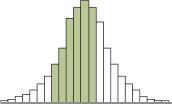
Thus, the area of these bars is the relative frequency in the interval of interest. In Chapter 5, we stated that we are using the relative frequency interpretation of probability. Therefore, the area shaded in the histogram will estimate the probability of the random variable being in that interval.
Now, let’s think of all of the possible data in the population. In this case, we can shrink the width of the bars to however small we wish. As we let the bar widths shrink to zero, then we end up with a smooth curve like below.
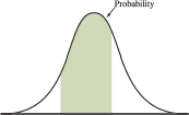
The smooth curve (probability distribution of a continuous random variable) is denoted by the symbol \(f(x)\) and is often called the probability density function (pdf). We can still view the area of the shaded region as the probability.
Because the area under the pdf represents probability, then by definition we have \[ P(X=x)=0 \] In other words, we assign a probability of zero at a point. This happens since there is no area under the curve at a point.
We do find the probability of a continuous random variable in an interval: \[ P(a< X< b) \] How do we do this? We find the area under the curve between \(a\) and \(b\). We find the area under the curve by taking the integral \[ P(a < X < b) = \int_a^b f(x) \; dx. \]
The cumulative distribution function (cdf) of \(X\), denoted \(F(x)\), gives the probability that \(X\) is less than or equal to \(x\); it is the area under the density to the left of \(x\).
In summary:
The probability distribution of a continuous random variable \(X\)
- is represented by a smooth curve
- the curve is called the probability density function (pdf)
- the probability \(P(a<X<b)=P(a\le X\le b)\) is the area under the curve between \(a\) and \(b\)
- the cumulative distribution function (cdf) give the area to the left of some value: \(F(x)=P(X\le x)\)
ExampleExample 7.1: Drug Metabolism
After an oral dose, the amount of a drug in the bloodstream rises and then falls over time. If we pick a random patient and record their peak plasma concentration, that value could be any number within a physiological range.
The probability that the peak is exactly 3.000 µg/mL is zero; but we can talk meaningfully about the probability it lies between 2.8 and 3.2 µg/mL, which is the area under the density between those points.
ExampleExample 7.2: Component lifetime in manufacturing
An electronics manufacturer measures the operating lifetime (in hours) of a certain type of capacitor. Because the lifetime can take any positive value (1,203.7 hours, 1,203.71 hours, and so on) it is modeled as a continuous random variable. A quality engineer might ask: what is the probability that a randomly selected capacitor lasts longer than 1,500 hours? The answer is the area under the density curve to the right of 1,500.
When interpreting a probability density function for a continuous random variable, it is crucial to remember what the graph is, and what it is not, telling you.
A pdf does not give the probability of a specific value. Instead, it describes how probability is distributed across an interval. The vertical axis represents probability density, not probability itself. As a result, a taller portion of the curve indicates a region where probability is more densely concentrated, but the probability of any single exact value is still zero.
A helpful analogy is to think of the pdf like a topographic map. A taller peak indicates where probability is concentrated, but the “amount” of probability depends on how wide that region is. A very tall but extremely narrow spike may contribute little total probability because its area is small.
Mean, Variance, and Standard Deviation of a Continuous Random Variable
Recall that for a discrete random variable, the mean and variance are computed using weighted sums over all possible values:
\[ \mu = \sum_x x \cdot P(X=x), \qquad \sigma^2 = \sum_x (x-\mu)^2 \cdot P(X=x). \]
Each term multiplies a value of \(X\) by its probability, then adds everything up.
For a continuous random variable, the same idea applies — we still compute a weighted average, but because \(X\) can take infinitely many values in an interval and \(P(X = a) = 0\) for any single point, there is nothing meaningful to “add up” at individual values. The natural replacement for a sum over infinitely many points is an integral, a concept from calculus.
The formulas for the mean and variance of a continuous random variable are:
\[ \mu = \int_{-\infty}^{\infty} x \, f(x) \, dx, \qquad \sigma^2 = \int_{-\infty}^{\infty} (x - \mu)^2 \, f(x) \, dx. \]
The structure mirrors the discrete case exactly — each value of \(x\) is weighted by the density \(f(x)\), and the integral accumulates those contributions across all possible values. Evaluating these integrals requires calculus and is beyond the scope of this course. For the distributions we study (the uniform and normal), the mean and standard deviation are given directly by convenient formulas, so you will not need to compute these integrals yourself.
The key takeaway is the conceptual parallel:
| Discrete | Continuous | |
|---|---|---|
| Mean | \(\sum x \cdot P(X=x)\) | \(\int x \cdot f(x)\,dx\) |
| Variance | \(\sum (x-\mu)^2 \cdot P(X=x)\) | \(\int (x-\mu)^2 \cdot f(x)\,dx\) |
| Tool | weighted sum | weighted integral |
Both compute a weighted average of the values of \(X\), weighted by how likely those values are. The integral is simply the continuous analogue of the sum.
Recap
| Keyword | Definition |
|---|---|
| continuous random variable | A random variable that can take any value in an interval; probabilities are assigned to ranges of values rather than individual points. |
| probability density function (PDF) | A non‑negative function \(f(x)\) such that \(P(a ≤ X ≤ b)\) equals the area under \(f(x)\) between \(a\) and \(b\) and the total area under the curve of \(f(x)\) is one. |
| cumulative distribution function (CDF) | The function \(F(x)=P(X ≤ x)\) giving the area under the PDF to the left of \(x\). It increases from 0 to 1 as \(x\) goes from \(-∞\) to \(∞\). |
Check your understanding
NoteProblems
- Explain in your own words why the probability that a continuous random variable equals exactly 5 is zero. How, then, do we assign probabilities for continuous variables?
- Sketch or describe the shape of a PDF that would model serum cholesterol levels in a population. Why can’t a PDF ever dip below the horizontal axis?
TipSolutions
- A continuous random variable can take infinitely many values within any interval. Because the PDF spreads probability continuously across these values, the probability of landing on any single point is zero. We obtain meaningful probabilities by integrating the density over an interval to find the area under the curve between the limits.
- Serum cholesterol tends to cluster around an average value with fewer extremely low or high values. A plausible PDF would be unimodal and right‑skewed: low near 0, rising to a peak near the typical cholesterol level, and gradually decreasing. The density must always stay at or above zero because probabilities cannot be negative.
7.2 The Uniform Distribution
“Don’t mistake possibilities for probabilities. Anything is possible. It’s the probabilities that matter” – Ray Dalio
The simplest continuous distribution is the uniform distribution. Imagine selecting a time uniformly at random within a two‑hour window; any minute in that window is just as likely as any other. More formally, a continuous random variable \(X\) has a Uniform\((c,d)\) distribution if its PDF is constant on the interval \((c,d)\) and zero elsewhere.
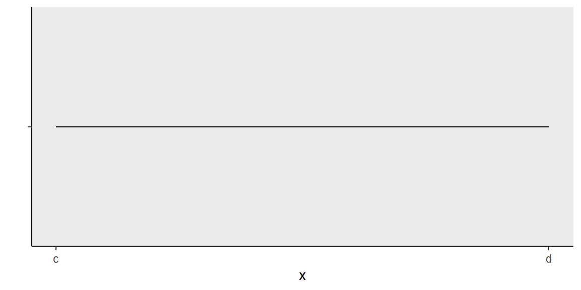
Since all values in the interval \((c,d)\) are equally likely, the pdf of a uniform random variable appears as a horizontal line:
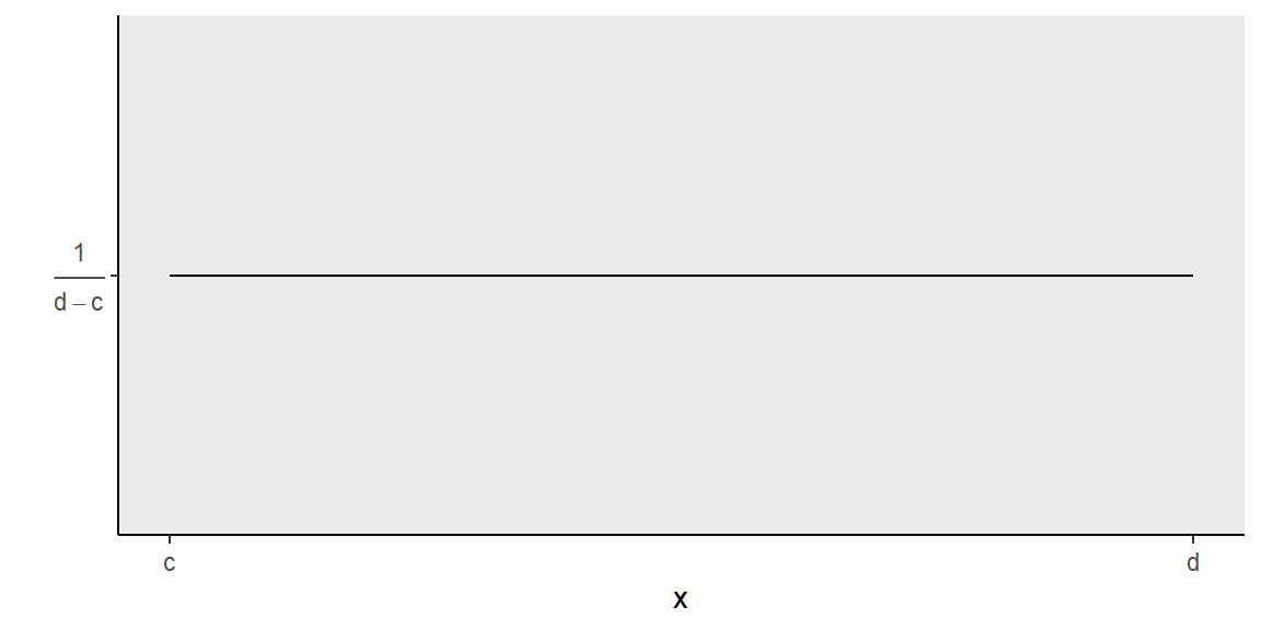
Note that the area under the curve must equal 1 (since the area corresponds to probability). Therefore, the area between \(c\) and \(d\) \[ \begin{align*} \text{area of rectangle} = \text{base}\times \text{height} &\Longrightarrow{ 1 = (d-c) \times \text{height}}\\\\ &\Longrightarrow \text{height} = \frac{1}{d-c} \end{align*} \]
So, the pdf of a uniform random variable is \[ f(x) = \frac{1}{d-c} \]
For a Uniform\((c,d)\) random variable, the key formulas are:
\[ \mu = \frac{c+d}{2}, \qquad \sigma^2 = \frac{(d-c)^2}{12}, \qquad \sigma = \frac{d-c}{\sqrt{12}} \]
The mean is simply the midpoint of the interval, which makes intuitive sense: if all values are equally likely, the average should land right in the middle. The variance captures how spread out the values are across the interval.
For finding a probability, because the density is flat at height \(\frac{1}{d-c}\), the probability of falling in any sub-interval \((a, b)\) within \((c, d)\) is just the length of that sub-interval divided by the total length:
\[ P(a < X < b) = \frac{b - a}{d - c} \]
TipFor those who want to see the math:
The mean follows from the definition \(\mu = \int_{-\infty}^{\infty} x f(x)\,dx\). Since \(f(x) = \frac{1}{d-c}\) on \((c,d)\) and zero elsewhere:
\[ \begin{align*} \mu &= \int_c^d x \cdot \frac{1}{d-c}\,dx\\ &= \frac{1}{d-c} \cdot \frac{x^2}{2}\Bigg|_c^d\\ &= \frac{1}{d-c} \cdot \frac{d^2 - c^2}{2}\\ &= \frac{(d-c)(d+c)}{2(d-c)}\\ &= \frac{c+d}{2} \end{align*} \]
The variance follows from \(\sigma^2 = \int_c^d (x-\mu)^2 \frac{1}{d-c}\,dx\), which after substituting \(u = x - \frac{c+d}{2}\) and integrating evaluates to \(\frac{(d-c)^2}{12}\).
The probability formula follows directly from integration:
\[ \begin{align*} P(a < X < b) &= \int_a^b \frac{1}{d-c}\,dx\\ &= \frac{1}{d-c}\,x\Big|_a^b\\ &= \frac{b-a}{d-c} \end{align*} \]
Summary of Uniform RVs:
- the pdf is \(f(x)=\frac{1}{d-c}\qquad c\le X\le d\)
- the mean is \(\mu = \frac{c+d}{2}\) and the standard deviation is \(\sigma=\frac{d-c}{\sqrt{12}}\)
- \(P(a<X<b)=\frac{b-a}{d-c}\)
ExampleExample 7.3: Stadium gate opening
A professional soccer team opens its stadium gates exactly 90 minutes before kickoff. Fans who arrive during that window tend to enter at random, with no particular time being more popular than any other. Let \(T\) be the number of minutes after the gates open when a randomly selected fan enters. Then \(T \sim \text{Uniform}(0, 90)\).
The mean arrival time is \[ \mu = \frac{0 + 90}{2} = 45 \text{ minutes after gate opening} \]
The standard deviation is \[ \sigma = \frac{90 - 0}{\sqrt{12}} \approx 25.98 \text{ minutes} \]
The probability that a fan arrives in the first 30 minutes (before the stadium fills up) is \[ P(0 \le T \le 30) = \frac{30 - 0}{90 - 0} = \frac{30}{90} \approx 0.333 \]
About 33% of fans are expected to arrive within the first 30 minutes of the gates opening.
ExampleExample 7.4: Machine calibration error
A precision milling machine produces metal parts whose lengths are designed to be exactly 50 mm. Due to natural mechanical variation, the actual length of any given part is equally likely to fall anywhere in the range \([49.6, 50.4]\) mm. Let \(X \sim \text{Uniform}(49.6, 50.4)\) be the length of a randomly selected part.
The mean length is \[ \mu = \frac{49.6 + 50.4}{2} = 50.0 \text{ mm} \]
The standard deviation is \[ \sigma = \frac{50.4 - 49.6}{\sqrt{12}} = \frac{0.8}{\sqrt{12}} \approx 0.231 \text{ mm} \]
Parts outside the tolerance range \([49.7, 50.3]\) mm are considered defective. The probability that a part is defective is \[ \begin{align*} P(X < 49.7 \text{ or } X > 50.3) &= 1 - P(49.7 \le X \le 50.3)\\ &= 1 - \frac{50.3 - 49.7}{50.4 - 49.6}\\ &= 1 - \frac{0.6}{0.8}\\ &= 0.25 \end{align*} \]
Under this model, 25% of parts fall outside the tolerance range.
Computing Uniform Probabilities in R
R provides four built-in functions for working with the uniform distribution, following the same naming convention as the binomial functions:
| Function | What it computes |
|---|---|
dunif(x, min, max) |
The density \(f(x) = \frac{1}{\text{max} - \text{min}}\) at a point \(x\) |
punif(q, min, max) |
\(P(X \le q)\): the cumulative probability up to \(q\) |
qunif(p, min, max) |
The value \(x\) such that \(P(X \le x) = p\) (the quantile function) |
runif(n, min, max) |
Generates \(n\) random draws from \(\text{Uniform}(\text{min}, \text{max})\) |
The code below reproduces the calculations from Examples 7.3 and 7.4.
# Example 7.3: Stadium gate opening -- T ~ Uniform(0, 90)
# P(0 <= T <= 30): fan arrives in first 30 minutes
punif(30, min = 0, max = 90)
[1] 0.3333333# Example 7.4: Machine calibration -- X ~ Uniform(49.6, 50.4)
# P(49.7 <= X <= 50.3): part is within tolerance
punif(50.3, min = 49.6, max = 50.4) - punif(49.7, min = 49.6, max = 50.4)[1] 0.75# P(defective): outside tolerance
1 - (punif(50.3, min = 49.6, max = 50.4) - punif(49.7, min = 49.6, max = 50.4))[1] 0.25# What length do only the top 10% of parts exceed? (90th percentile)
qunif(0.90, min = 49.6, max = 50.4)[1] 50.32You can also simulate uniform data with runif(). For example, simulating 10,000 machine parts and checking what fraction are defective:
library(tidyverse)

set.seed(42)
parts <- tibble(length = runif(10000, min = 49.6, max = 50.4))

parts |>
  summarise(
    pct_defective = mean(length < 49.7 | length > 50.3)
  )
# A tibble: 1 × 1
pct_defective
<dbl>
1 0.255Recap
| Keyword | Definition |
|---|---|
| uniform distribution | A continuous distribution on \((c,d)\) whose PDF is constant at height \(1/(d-c)\). All intervals of equal length within \((c,d)\) have equal probability. |
Check your understanding
NoteProblems
- Suppose \(X\sim\text{Uniform}(0,10)\). What is \(P(3 ≤ X ≤ 7)\)? Explain your reasoning.
- A researcher measures the pH of soil samples collected uniformly at random along a transect from 0 to 100 m. What is the probability that a randomly selected soil sample comes from between 20 m and 35 m? Express your answer numerically.
- If \(Y\sim\text{Uniform}(c,d)\) and you know that \(P(Y ≤ 5) = 0.5\), what relationship does this imply between \(c\), \(d\) and 5?
TipSolutions
- The interval from 3 to 7 has length 4. Since the distribution is Uniform\((0,10)\), the probability of any subinterval equals its length divided by the total length: \(4/10=0.4\).
- The transect is 100 m long. The segment from 20 to 35 m is 15 m long, so \(P(20 ≤ X ≤ 35) = 15/100 = 0.15\).
- For a uniform distribution, \(P(Y ≤ y) = (y-c)/(d-c)\) for \(c ≤ y ≤ d\). Setting \(P(Y≤5)=0.5\) implies \((5 - c)/(d - c) = 0.5\). Equivalently, \(5\) is the midpoint of the interval and \(5 = (c + d)/2\).
7.3 The Normal Distribution
“the normal distribution is seldom, if ever, observed in nature.” – Louis Guttman
The normal distribution (also called the Gaussian distribution) is the most celebrated continuous distribution in statistics. It appears throughout science, engineering, and the social sciences and forms the theoretical backbone of many statistical procedures, including confidence intervals, hypothesis tests, and regression methods.
Basic shape and properties
A random variable with distribution \(N(\mu,\sigma)\) has a density curve that is:
- symmetric about \(\mu\),
- bell-shaped (unimodal with a single peak),
- and continuous over the entire real line.
Because of the symmetry,
\[ \text{mean} = \text{median} = \text{mode} = \mu. \]
The curve extends infinitely in both directions, getting closer and closer to the horizontal axis but never actually touching it. Thus, in theory, any real number is possible, although values far from the mean have very small probability density.
The parameters \(\mu\) and \(\sigma\)
The normal distribution is completely determined by two parameters:
- \(\mu\) (mu): the location parameter, which sets the center of the distribution.
- \(\sigma\) (sigma): the scale parameter, which determines the spread.
More specifically:
- \(\mu\) is the location of the peak and the balance point of the distribution.
- \(\sigma\) is the standard deviation and controls the width of the bell.
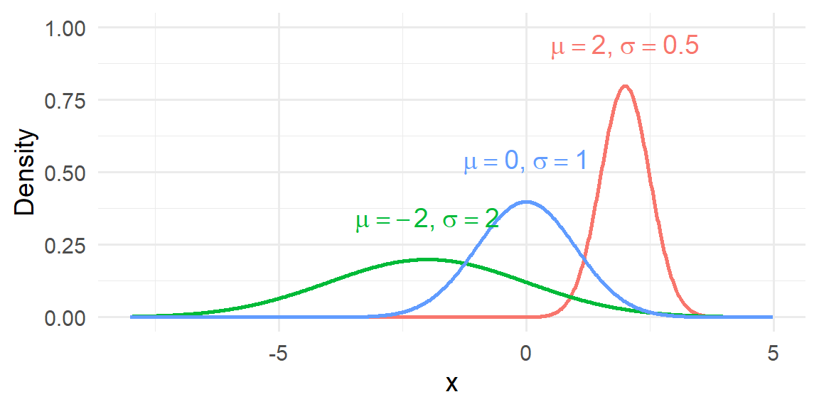
Changing \(\mu\) shifts the entire curve left or right without altering its shape. Changing \(\sigma\) stretches or compresses the curve:
- Larger \(\sigma\) → wider, flatter bell
- Smaller \(\sigma\) → narrower, taller bell
The Normal Probability Density Function
The probability density function (pdf) of a normal random variable is
\[ f(x) = \frac{1}{\sigma\sqrt{2\pi}} \exp\left(-\frac{(x-\mu)^2}{2\sigma^2}\right), \qquad -\infty < x < \infty. \]
While this formula looks complicated, its key role is to produce the familiar bell-shaped curve and to ensure that the total area under the curve equals 1.
You do not need to memorize this formula to use the normal model. More important are its qualitative properties: it is unimodal, symmetric, and tails off smoothly; the total area under the curve is one.
Why the normal distribution matters
The normal distribution occupies a special place in statistics not because every dataset is normal—many are not—but because the normal model emerges naturally in a wide range of settings and underpins much of statistical theory and practice.
Several key reasons explain its importance:
Many natural phenomena are approximately normal. Measurements such as adult heights, measurement errors in instruments, and certain biological traits often display the familiar symmetric, bell-shaped pattern. This occurs because the observed value is frequently the result of many small, independent influences acting together. When no single factor dominates, the combined effect tends to produce a roughly normal distribution.
Sample means are often approximately normal (Central Limit Theorem). Perhaps the most powerful reason for the normal distribution’s prominence is the Central Limit Theorem (CLT). Roughly speaking, the CLT states that the distribution of the sample mean becomes approximately normal as the sample size grows, regardless of the shape of the original population (provided certain mild conditions hold). This remarkable result allows statisticians to use normal-based methods even when the underlying data are skewed or irregular. We will discuss the Central Limit Theorem more thouroughly in Chapter 8.
Many statistical methods rely on normal approximations. Classical inference procedures—such as z-tests, many confidence intervals, regression inference, and numerous quality-control methods—are derived under normal assumptions or justified by the CLT. The mathematics of the normal distribution is especially tractable, which makes it a convenient and powerful modeling tool.
Beyond these points, the normal distribution also serves as a benchmark model. Analysts often begin by comparing their data to a normal curve to assess symmetry, detect skewness, or identify heavy tails. Even when the normal model is not ultimately appropriate, it provides a useful reference point for understanding the data’s structure.
Importantly, real-world data are rarely perfectly normal. They may be skewed, have heavier tails, or exhibit multiple peaks. Nevertheless, the normal model often provides a useful first approximation, especially for averages and measurement error, and it forms the conceptual and mathematical foundation for many more advanced statistical techniques.
In short, the normal distribution matters not because it fits everything perfectly, but because it appears frequently, behaves predictably, and enables a vast toolkit of statistical methods.
Graphing the Normal Distribution in R
The dnorm(x, mean, sd) function returns the height of the normal density curve at a given value of x. To draw a smooth curve with ggplot2, we generate a dense sequence of x values, compute the density at each one, and plot them as a line.
The example below draws the \(N(70, 3)\) distribution (representing, say, exam scores with a mean of 70 and a standard deviation of 3) and shades the region within one standard deviation of the mean.
library(tidyverse)

mu <- 70
sigma <- 3

curve_data <- tibble(
  x       = seq(mu - 4 * sigma, mu + 4 * sigma, length.out = 500),
  density = dnorm(x, mean = mu, sd = sigma)
)

ggplot(curve_data, aes(x = x, y = density)) +
  geom_line(linewidth = 1) +
  geom_area(
    data = filter(curve_data, x >= mu - sigma, x <= mu + sigma),
    fill = "#2c7fb8", alpha = 0.4
  ) +
  labs(
    x = "Score", y = "Density",
    title = "Normal distribution: N(70, 3)",
    subtitle = "Shaded region: within 1 SD of the mean (~68%)"
  ) +
  theme_minimal()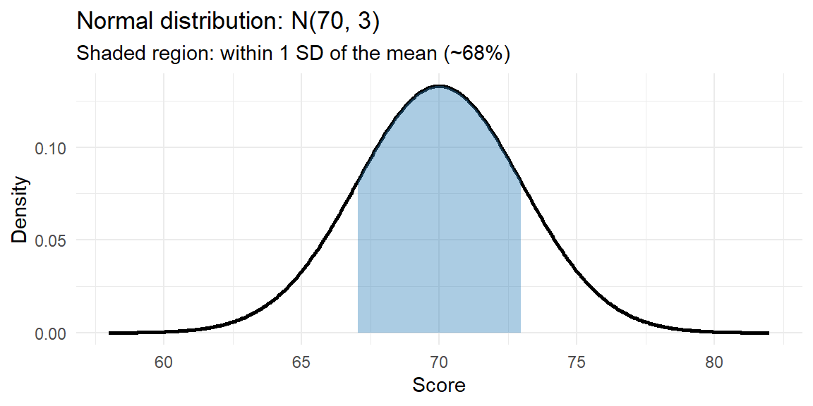
Recap
| Keyword | Definition |
|---|---|
| normal distribution | A continuous, symmetric bell‑shaped distribution defined by its mean \(\mu\) and standard deviation \(\sigma\); mean = median = mode. |
| standard normal distribution | The special case Normal\((0,1)\); its values are often called z‑scores, and any normal distribution can be standardized via \(z = (x - \mu)/\sigma\). |
Check your understanding
NoteProblems
- What does it mean that the mean, median and mode of a normal distribution are equal? How is this reflected in the shape of the curve?
- For a \(N(150,20)\) distribution (representing, say, birth weights in grams), approximately what percentage of babies weigh between 110 g and 190 g?
- Explain why extreme values (more than 3 standard deviations from the mean) are considered unusual under the normal model.
TipSolutions
- A normal curve is perfectly symmetric about its mean; the highest point occurs at \(\mu\) and the curve declines equally on both sides. Because of this symmetry, the most typical value (the mode), the point dividing the distribution in half (the median) and the arithmetic average (the mean) coincide.
- Two standard deviations on either side of the mean cover about 95% of the data. The interval from \(\mu-2\sigma = 150 - 40 = 110\) to \(\mu+2\sigma = 190\) therefore captures roughly 95% of birth weights.
- Under the normal model, only about 0.3% of observations lie beyond three standard deviations from the mean by the empirical rule. Thus values outside that range are rare and often signal measurement error or a departure from normality.
7.4 Finding Probability for a Normal Distribution
“I once worked with a guy for three years and never learned his name. Best friend I ever had. We still never talk sometimes.” -Ron Swanson
Once we determine the normal model for a variable, we can compute probabilities using R’s pnorm() function. Given \(X\sim N(\mu,\sigma)\), pnorm(x, mean, sd) returns \(P(X \le x)\) — the area under the curve to the left of x. All other normal probability types are derived from this.
The z‑score \(z = (x - \mu)/\sigma\) measures how many standard deviations a value is from the mean. Standardizing converts any \(N(\mu, \sigma)\) probability to an equivalent \(N(0,1)\) calculation, but pnorm() handles any \(\mu\) and \(\sigma\) directly so you rarely need to standardize by hand.
Types of normal probability problems
| Probability | R expression |
|---|---|
| \(P(X < a)\) | pnorm(a, mean, sd) |
| \(P(X > a)\) | pnorm(a, mean, sd, lower.tail = FALSE) |
| \(P(a < X < b)\) | pnorm(b, mean, sd) - pnorm(a, mean, sd) |
| \(P(X < a \text{ or } X > b)\) | pnorm(a, mean, sd) + pnorm(b, mean, sd, lower.tail = FALSE) |
The examples below all use adult exam scores that follow a \(N(75, 8)\) distribution (mean 75, standard deviation 8).
Probability less than a value — \(P(X < 70)\)
pnorm(70, mean = 75, sd = 8)[1] 0.2659855About 26.6% of students score below 70.
Probability greater than a value — \(P(X > 85)\)
pnorm(85, mean = 75, sd = 8, lower.tail = FALSE)[1] 0.1056498About 10.6% of students score above 85.
Probability between two values — \(P(65 < X < 85)\)
pnorm(85, mean = 75, sd = 8) - pnorm(65, mean = 75, sd = 8)[1] 0.7887005About 78.9% of students score between 65 and 85.
Probability beyond two values (two tails) — \(P(X < 60 \text{ or } X > 90)\)
pnorm(60, mean = 75, sd = 8) + pnorm(90, mean = 75, sd = 8, lower.tail = FALSE)[1] 0.06079272About 6.1% of students score below 60 or above 90.
Probability beyond a number of standard deviations from the mean — \(P(|Z| > 2)\)
Recall that a z-score give the number of standard deviations from the mean a value is. Therefore, we can use the standard normal distribution.
pnorm(-2, mean = 0, sd = 1) +
  pnorm(2, mean = 0, sd = 1, lower.tail = FALSE)
[1] 0.04550026# Note that lower.tail = FALSE gives the area to the right. About 4.6% of scores fall more than 2 standard deviations from the mean. This matches the empirical rule’s statement that roughly 95% fall within 2 SDs, leaving about 5% in the two tails combined.
Probability within a number of standard deviations of the mean — \(P(|Z| < 1)\)
pnorm(1, mean = 0, sd = 1) - pnorm(-1, mean = 0, sd = 1)[1] 0.6826895About 68.3% of scores fall within 1 standard deviation of the mean — confirming the 68–95–99.7 empirical rule.
Recap
| Keyword | Definition |
|---|---|
| z‑score | The number of standard deviations a value \(x\) is from the mean: \(z=(x-\mu)/\sigma\). |
pnorm() |
R function returning \(P(X \le x)\) for a normal distribution; use lower.tail = FALSE for upper-tail probabilities. |
Note”Problems”
- Adult resting heart rates follow a \(N(72, 10)\) distribution (beats per minute). What is the probability that a randomly selected adult has a resting heart rate below 60?
- Using the same heart rate distribution, what is the probability of a heart rate above 90?
- What proportion of adults have a resting heart rate between 60 and 80?
- What proportion have a heart rate more than 2.5 standard deviations from the mean?
Tip”Solutions”
pnorm(60, mean = 72, sd = 10)\(\approx 0.1151\). About 11.5% of adults have a resting heart rate below 60 bpm.pnorm(90, mean = 72, sd = 10, lower.tail = FALSE)\(\approx 0.0359\). About 3.6% have a resting heart rate above 90 bpm.pnorm(80, mean = 72, sd = 10) - pnorm(60, mean = 72, sd = 10)\(\approx 0.673\). About 67.3% of adults fall in this range.pnorm(72 - 2.5*10, mean = 72, sd = 10) + pnorm(72 + 2.5*10, mean = 72, sd = 10, lower.tail = FALSE)\(\approx 0.0124\). About 1.2% of adults fall more than 2.5 SDs from the mean.
7.5 Finding a Quantile for a Normal Distribution
“Two things are infinite: the universe and human stupidity; and I’m not sure about the universe.” – Albert Einstein
In many applications we know a desired probability and wish to find the corresponding value of \(x\) such that \(P(X ≤ x)=p\). This value is called a quantile or percentile of the distribution. Mathematically, the quantile function \(F^{-1}(p)\) is the inverse of the cumulative distribution function. For a normal distribution, the quantile function returns the \(x\) value whose cumulative probability is \(p\).
Relationship between the CDF and quantiles
The cumulative distribution function \(F(x)\) gives the probability that a random variable \(X\) is less than or equal to \(x\). The quantile function does the reverse: it takes a probability \(p\) and returns the threshold \(x\) such that \(P(X ≤ x)=p\). For example, the 0.5 quantile is the median. Because the normal CDF does not have a simple algebraic inverse, quantiles are typically obtained from tables or software.
At times, there are special quantiles that will show up in statistical methods that we will discuss later. We denote these as \[ p = P(Z> z_p) \] In other words, \(z_p\) is the value of the standard normal distribution that will have \(p\) area to the right. For example, \(z_{0.05}\) is the value that has 0.05 area to the right.
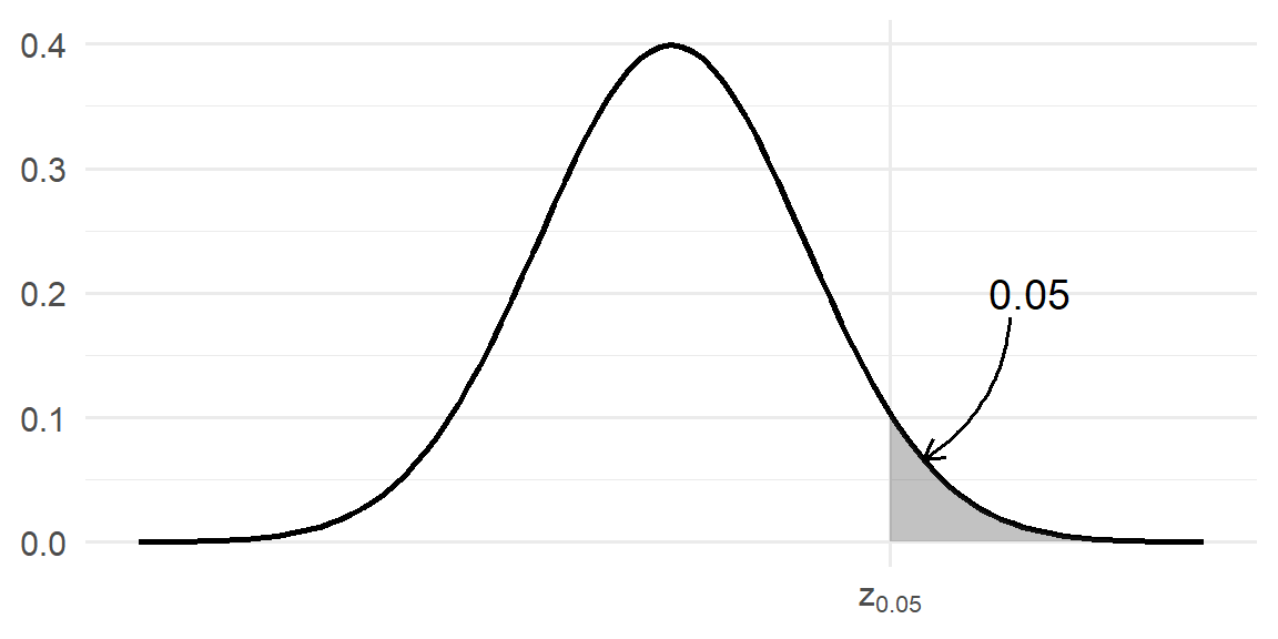
Here the value is \[ z_{0.05}=1.645 \]
Finding Quantiles with R
The qnorm() function is the inverse of pnorm(): given a cumulative probability \(p\), it returns the value \(x\) such that \(P(X \le x) = p\).
qnorm(p, mean, sd)               # x such that P(X <= x) = p
qnorm(p, mean, sd, lower.tail = FALSE)  # x such that P(X > x) = p
The examples below continue with exam scores distributed \(N(75, 8)\).
Find a lower-tail percentile — What score marks the bottom 10% of students?
qnorm(0.10, mean = 75, sd = 8)[1] 64.74759A score of about 64.7 is the 10th percentile: 10% of students score below this.
Find an upper-tail cutoff — What score do only the top 5% of students exceed?
qnorm(0.95, mean = 75, sd = 8)[1] 88.15883A score of about 88.2 is the 95th percentile; only 5% of students score above it.
Find the bounds of the middle 95% — Between what two scores do 95% of students fall?
qnorm(0.025, mean = 75, sd = 8) # lower bound[1] 59.32029qnorm(0.975, mean = 75, sd = 8) # upper bound[1] 90.67971The central 95% of scores falls between approximately 59.3 and 90.7.
Find the bounds of the middle 68% — Between what two scores do about 68% of students fall?
qnorm(0.16, mean = 75, sd = 8)[1] 67.04434qnorm(0.84, mean = 75, sd = 8)[1] 82.95566This confirms the empirical rule: about 68% of students score within roughly one standard deviation of the mean (between 67 and 83).
Find a critical z-value — What is \(z_{0.05}\), the standard normal value with 5% area to the right?
qnorm(0.05, lower.tail = FALSE) # or equivalently: qnorm(0.95)[1] 1.644854\(z_{0.05} \approx 1.645\), confirming the value shown in the plot above.
ExampleExample 7.5: therapeutic drug monitoring
Suppose therapeutic blood levels of a drug follow a \(N(50, 10)\) distribution. Physicians want to flag concentrations above the 97.5th percentile as potentially dangerous. What threshold should they use?
qnorm(0.975, mean = 50, sd = 10)[1] 69.59964The 97.5th percentile is approximately 69.6 ng/mL. Only 2.5% of patients are expected to have concentrations above this value; concentrations exceeding it may warrant clinical review.
To verify, we can confirm that pnorm(69.6, mean = 50, sd = 10, lower.tail = FALSE) returns approximately 0.025.
pnorm(69.6, mean = 50, sd = 10, lower.tail = FALSE)[1] 0.0249979Recap
| Keyword | Definition |
|---|---|
| quantile (percentile) | For a continuous distribution with CDF \(F\), the value \(x = F^{-1}(p)\) such that \(P(X \le x) = p\). |
qnorm() |
R function returning the quantile \(x\) for a given cumulative probability \(p\); the inverse of pnorm(). |
Check your understanding
NoteProblems
- Adult resting heart rates follow a \(N(72, 10)\) distribution. What heart rate marks the top 15% of the population? Use
qnorm(). - Using the same distribution, find the heart rate interval that contains the central 90% of the population.
- Explain in your own words the relationship between
pnorm()andqnorm(). Ifpnorm(85, mean = 72, sd = 10)returns some value \(p\), what wouldqnorm(p, mean = 72, sd = 10)return?
TipSolutions
- The top 15% corresponds to the 85th percentile:
qnorm(0.85, mean = 72, sd = 10)\(\approx 82.4\) bpm. Only 15% of adults have a resting heart rate above approximately 82.4 bpm. - The central 90% lies between the 5th and 95th percentiles:
qnorm(0.05, mean = 72, sd = 10)\(\approx 55.6\) andqnorm(0.95, mean = 72, sd = 10)\(\approx 88.4\). About 90% of adults have resting heart rates between 55.6 and 88.4 bpm. pnorm()andqnorm()are inverses of each other.pnorm(x)takes a value and returns a probability;qnorm(p)takes a probability and returns the value. Soqnorm(pnorm(85, mean = 72, sd = 10), mean = 72, sd = 10)would return 85.