12Methods for Quantitative Response Variables – One and Two Groups
“It’s easy to lie with statistics. It’s hard to tell the truth without statistics.” – Andrejs Dunkels
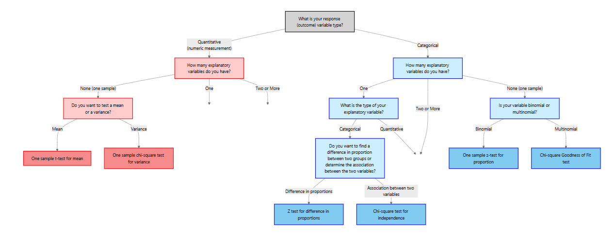
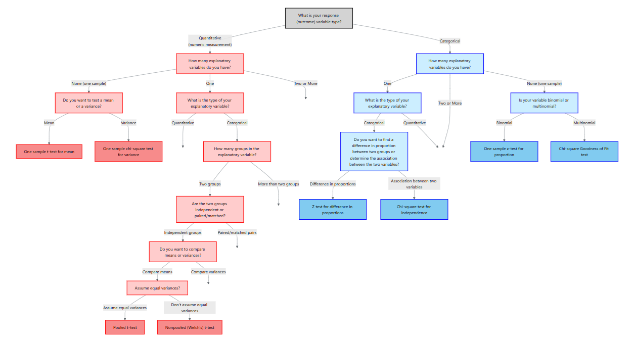
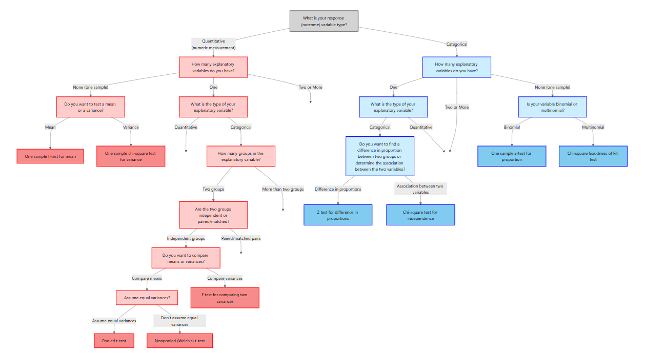
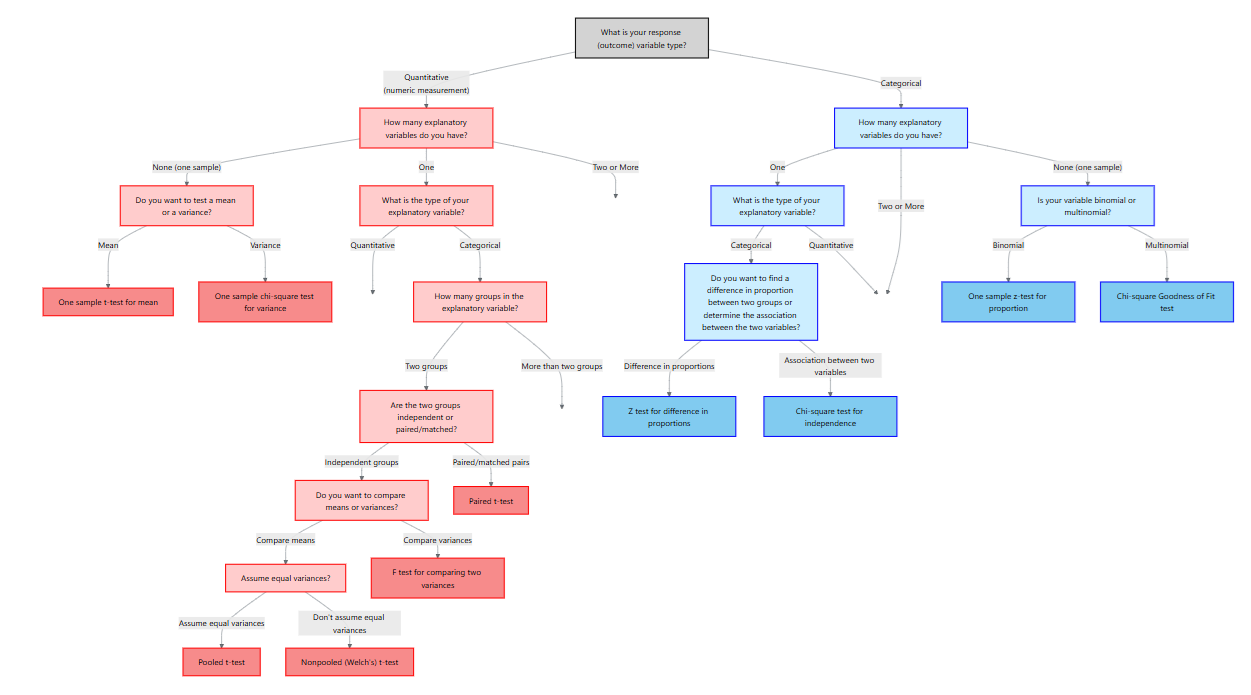
In the previous chapter we focused on categorical outcomes. Here our response variable is quantitative, meaning it is measured on a numeric scale such as weight, blood pressure, cholesterol level, enzyme activity, revenue or time. To decide on an appropriate analysis we must consider how many explanatory variables we have and whether the data are paired or independent. The table below summarizes the situations covered in this chapter:
Scenario
Response variable
Explanatory variable
Appropriate method
No explanatory variable
Quantitative
None (one sample)
One‑sample t‑test for the mean and chi‑square test for the variance
Two paired measurements
Quantitative
One categorical variable with two matched levels (e.g., before/after on the same subject)
Paired t‑test
Two independent groups
Quantitative
One categorical variable with two independent levels (e.g., treatment vs. control)
Two‑sample t‑test for means (pooled or Welch) and F‑test for equality of variances
12.1 One‑Sample Tests for the Mean and Variance
When there is no explanatory variable, we have a single quantitative sample. Two natural questions arise:
Is the population mean equal to a specified value?
Is the population variance equal to a specified value?
We address these with the one‑sample t-test and the chi‑square test for the variance.
One‑sample t‑test for a mean
Suppose we have a random sample \(x_1, x_2,\dots,x_n\) from a population with unknown mean \(\mu\) and standard deviation \(\sigma\). We want to test
Like all inference methods, the t‑test rests on assumptions. In practice we require:
A simple random sample from the population of interest; observations are independent of one another.
The population is normally distributed, or the sample size is large (typically \(n \ge 30\)) so that the Central Limit Theorem ensures approximate normality.
Test statistic and p‑value
Under \(H_0\), the test statistic
\[
t = \frac{\bar{x} - \mu_0}{s/\sqrt{n}}
\]
follows a Student’s \(t\) distribution with \(n-1\) degrees of freedom. We obtain the p‑value by comparing the observed \(|t|\) to the \(t\) distribution. For a two‑sided alternative the p‑value is \(2P(T_{n-1} > |t|)\); for a one‑sided alternative we compute \(P(T_{n-1} > t)\) or \(P(T_{n-1} < t)\) depending on the direction.
Confidence interval
When the test is significant (or even when it is not), a \((1-\alpha)\times100\%\) confidence interval for \(\mu\) gives a range of plausible values. The interval is
where \(t_{\alpha/2}\) is the critical value from the \(t\) distribution.
ExampleExample 12.1: Monthly Fund Returns
A financial analyst reviews 15 months of returns for an actively managed mutual fund. The sample mean return is 3.4% with a standard deviation of 0.6%. The benchmark index averages 3.0% per month. Test whether the fund’s mean monthly return differs from the benchmark at the 5% significance level.
Solution. The hypotheses are \(H_0: \mu = 3.0\) vs. \(H_a: \mu \neq 3.0\). The test statistic is
\[
t = \frac{3.4 - 3.0}{0.6/\sqrt{15}} \approx 2.58.
\]
With \(n-1 = 14\) degrees of freedom the two‑sided p‑value is \(2P(T_{14} > 2.58) \approx 0.021\). Since 0.021 < 0.05, we reject \(H_0\) and conclude that the fund’s mean monthly return differs from the 3.0% benchmark. A 95% confidence interval is \(3.4 \pm t_{0.025,14}\times0.6/\sqrt{15} = (3.05, 3.75)\).
We can reproduce this in R:
set.seed(10040000)#simulate the data since all we have are summary statsreturns <-rnorm(15, mean =3.4, sd =0.6)t.test(returns, mu =3.0, alternative ="two.sided")
    One Sample t-test

data:  returns
t = 2.5764, df = 14, p-value = 0.02196
alternative hypothesis: true mean is not equal to 3
95 percent confidence interval:
 3.071913 3.786693
sample estimates:
mean of x
 3.429303
Performing the one-sample mean test in R
Use t.test() with a numeric vector and the hypothesized mean:
# Example: test whether mean monthly return differs from 3.0%# x = your data vector# mu = hypothesized population mean# alternative = "two.sided", "greater", or "less"t.test(returns, mu =3.0, alternative ="two.sided")
    One Sample t-test

data:  returns
t = 2.5764, df = 14, p-value = 0.02196
alternative hypothesis: true mean is not equal to 3
95 percent confidence interval:
 3.071913 3.786693
sample estimates:
mean of x
 3.429303
The output reports the t statistic, degrees of freedom, p-value, sample mean, and a confidence interval for \(\mu\). Change alternative to "greater" or "less" for a one-sided test.
Chi‑square test for a variance
Sometimes we are interested in assessing whether the population variance equals a specified value \(\sigma_0^2\). For example, an engineer may want to know whether the variability of machine parts exceeds a tolerance level. Let \(s^2\) be the sample variance computed from a random sample of size \(n\). To test
which has a chi‑square distribution with \(n-1\) degrees of freedom under \(H_0\). Large values of \(\chi^2\) indicate that \(s^2\) is bigger than expected under \(H_0\); small values indicate it is too small. For a two‑sided alternative the p‑value is \(P(\chi^2_{n-1} > \chi^2_\text{obs})\) for one tail plus \(P(\chi^2_{n-1} < \chi^2_\text{obs})\) for the other.
Confidence interval
A \((1-\alpha)\times100\%\) confidence interval for the population variance is
where \(\chi^2_{\alpha/2, n-1}\) and \(\chi^2_{1-\alpha/2, n-1}\) are critical values from the chi‑square distribution. Taking square roots yields a confidence interval for the standard deviation.
ExampleExample 12.2: Manufacturing Variability
A company manufactures springs with a target variance in spring length of \(\sigma_0^2 = 0.04\ \mathrm{cm}^2\). A quality‑control engineer measures 25 springs and computes a sample variance of \(s^2 = 0.065\ \mathrm{cm}^2\). Test whether the variance differs from the target at the 5% level.
Solution. With \(n-1 = 24\) degrees of freedom, the test statistic is \[
\begin{align*}
\chi^2 &= \frac{(24)(0.065)}{0.04}\\
&= 39.0
\end{align*}
\]
For a two‑sided test, the p‑value is about \(2P(\chi^2>39.0)=0.055\). We fail to reject \(H_0\). A 95% confidence interval for \(\sigma^2\) is
A sporting goods manufacturer claims its premium basketball averages 29.5 inches in circumference. A quality inspector measures 12 randomly selected basketballs and finds a sample mean of 29.2 inches with a standard deviation of 0.4 inches. At \(\alpha=0.05\) test whether the average circumference differs from 29.5 inches and compute a 95% confidence interval.
An economist studying quarterly GDP growth in 16 emerging markets obtains a sample variance of \(s^2=0.25\) percentage points². Test whether the true variance differs from 0.20 at \(\alpha=0.10\).
Why does the t‑test for the mean use the sample standard deviation \(s\) in the denominator instead of the known standard deviation \(\sigma\)?
TipSolutions
Test of the mean:\(H_0: \mu=29.5\) vs. \(H_a: \mu\neq29.5\). Here \(\bar{x}=29.2\), \(s=0.4\) and \(n=12\), so \(t=(29.2-29.5)/(0.4/\sqrt{12})\approx-2.60\). With \(n-1=11\) df the two‑sided p‑value is \(2P(T_{11}>2.60)\approx0.025\). At \(\alpha=0.05\) we reject\(H_0\) and conclude the mean circumference differs from 29.5 inches. A 95% CI is \(29.2 \pm t_{0.025,11}\times0.4/\sqrt{12}=(28.95, 29.45)\).
With \(n-1=15\) df the test statistic is \(\chi^2=(15\times0.25)/0.20=18.75\). The critical values at \(\alpha=0.10\) are \(\chi^2_{0.95,15}\approx7.26\) and \(\chi^2_{0.05,15}\approx24.99\). Since 18.75 lies between these, we fail to reject \(H_0\). The data do not provide enough evidence that the variance differs from 0.20.
In practice we rarely know the population standard deviation \(\sigma\). The t‑test treats \(s\) as an estimate of \(\sigma\). Using \(s\) introduces additional uncertainty, so the sampling distribution becomes a t distribution rather than a normal distribution.
12.2 Two Independent Samples: Student’s t‑Test and Welch’s t‑Test
“The twin assumptions of normality of distribution and homogeneity of variance are not ever exactly fulfilled in practice, and often they do not even hold to a good approximation.” -John Tukey
When comparing means between two independent groups, the appropriate procedure depends on whether the population variances are equal. We consider two methods: the pooled (Student’s) t‑test and Welch’s t‑test.
Student’s (pooled) t‑test
Let \(x_{1i}\) and \(x_{2j}\) be independent random samples from populations with means \(\mu_1\) and \(\mu_2\) and common variance \(\sigma^2\). To test \[
\begin{align*}
&H_0: \mu_1 = \mu_2\\
&H_a: \mu_1 \neq \mu_2
\qquad\text{(or one‑sided)}
\end{align*}
\]
When the assumption of equal variances is violated, we use Welch’s t‑test (also called the nonpooled t-test). This test modifies the standard error and the degrees of freedom. The test statistic is
\[
t = \frac{\bar{x}_1 - \bar{x}_2}{\sqrt{s_1^2/n_1 + s_2^2/n_2}},
\]
This formula yields a non‑integer value; software uses it to compute the p‑value. The confidence interval for \(\mu_1 - \mu_2\) uses the same standard error and the \(t_{\nu}\) distribution.
Assumptions and choosing the test
The assumptions for two‑sample t‑tests: the groups must be independent, each sample should come from a normal distribution, and the variances should be equal for the pooled test. If variances are not equal, the Welch test is preferred. In practice, Welch’s t-test should be used by default unless it is known the variances are equal.
ExampleExample 12.3: Ad campaign effectiveness
A marketing analyst compares sales increases after two different advertising campaigns. Sales increases for 20 regions under campaign A have mean 1.8% and SD = 1.0%; for 18 regions under campaign B the mean is 1.2% with SD = 0.6%. We do not know if the population variances are equal so we use Welch’s t-test:
With \(\nu\approx31\) df, the two‑sided p‑value is 0.036. We reject \(H_0\); campaign A yields a greater increase in sales. A 95% CI for the difference is \((0.037, 1.163)\) percentage points.
We can replicate this in R:
set.seed(1004)campaign_A <-rnorm(20, mean =1.8, sd =1.0)campaign_B <-rnorm(18, mean =1.2, sd =0.6)# Welch's t-test (default; does not assume equal variances)t.test(campaign_A, campaign_B,alternative ="two.sided", var.equal =FALSE)
    Welch Two Sample t-test

data:  campaign_A and campaign_B
t = 2.6333, df = 30.429, p-value = 0.01317
alternative hypothesis: true difference in means is not equal to 0
95 percent confidence interval:
 0.1688933 1.3331008
sample estimates:
mean of x mean of y
 1.927982  1.176985
# Pooled t-test (use only if equal variances can be assumed)t.test(campaign_A, campaign_B,alternative ="two.sided", var.equal =TRUE)
    Two Sample t-test

data:  campaign_A and campaign_B
t = 2.56, df = 36, p-value = 0.01481
alternative hypothesis: true difference in means is not equal to 0
95 percent confidence interval:
 0.1560317 1.3459624
sample estimates:
mean of x mean of y
 1.927982  1.176985
Performing the two-sample tests in R
Pass two numeric vectors to t.test(). The key argument is var.equal:
    Welch Two Sample t-test

data:  campaign_A and campaign_B
t = 2.6333, df = 30.429, p-value = 0.01317
alternative hypothesis: true difference in means is not equal to 0
95 percent confidence interval:
 0.1688933 1.3331008
sample estimates:
mean of x mean of y
 1.927982  1.176985
Welch’s test (var.equal = FALSE) is the default and is recommended unless you have strong evidence that the population variances are equal.
Pooled test (var.equal = TRUE) assumes \(\sigma_1^2 = \sigma_2^2\); use only after confirming this with the F-test in the next section.
The output includes the Welch degrees of freedom, p-value, and a 95% confidence interval for \(\mu_1 - \mu_2\).
Tests \(H_0: \mu_1=\mu_2\) without assuming equal variances; statistic \((\bar{x}_1-\bar{x}_2)/\sqrt{s_1^2/n_1+s_2^2/n_2}\) with approximate df given by Welch’s formula.
Check your understanding
NoteProblems
A retail analyst compares the mean daily sales (in thousands of dollars) for two store formats. A sample of \(n=15\) urban stores has \(\bar{x}_1=110\) and \(s_1=12\); a sample of \(n=15\) suburban stores has \(\bar{x}_2=103\) and \(s_2=15\). Assume equal population variances. Test whether the mean daily sales differ at the 5% level and compute a 95% confidence interval for the difference.
TipSolutions
Since the F‑test is not significant, we use the pooled t‑test. The pooled standard deviation is \(s_p=\sqrt{(14\times12^2+14\times15^2)/28}=13.54\). The test statistic is \(t=(110-103)/(13.54\sqrt{1/15+1/15})=1.52\) with df = 28; the two‑sided p‑value is 0.14. We fail to reject \(H_0\); the mean daily sales do not differ significantly. A 95% CI is \((110-103) \pm t_{0.025,28}\,13.54\sqrt{2/15} = (-2.56, 16.56)\) thousand dollars.
12.3 Equality of Variances: F‑Test and Alternatives
“To make the preliminary test on variances is rather like putting to sea in a rowing boat to find out whether conditions are sufficiently calm for an ocean liner to leave port.” -George Box
The F‑test compares two sample variances to evaluate
Let \(s_1^2\) and \(s_2^2\) be the sample variances from independent random samples of sizes \(n_1\) and \(n_2\) drawn from normally distributed populations. Without loss of generality assume \(s_1^2 \ge s_2^2\). The test statistic
\[
F = \frac{s_1^2}{s_2^2}
\]
has an F distribution with \((n_1-1, n_2-1)\) degrees of freedom under \(H_0\). Large values of \(F\) indicate that \(s_1^2\) is much larger than \(s_2^2\); very small values (which correspond to \(s_2^2\) being larger) are captured by the symmetry of the F distribution.
Assumptions include:
Two independent random samples.
Each population is normally distributed. The F‑test is sensitive to departures from normality, so a normality check is essential.
Confidence interval for the ratio of variances
We can estimate the ratio of population variances \(\sigma_1^2/\sigma_2^2\) using the sample ratio \(F\) and obtain a \((1-\alpha)\times100\%\) confidence interval:
ExampleExample 12.4: Sprint time variability across training programs
A sports scientist compares the consistency of 40-yard dash times produced by two training programs. Program A (\(n_1=10\) athletes) yields a sample variance of \(s_1^2=0.08\) seconds²; Program B (\(n_2=12\) athletes) yields \(s_2^2=0.03\) seconds². A more consistent program produces less variability. With \(s_1^2 > s_2^2\), the test statistic is \(F=0.08/0.03=2.67\) with degrees of freedom \((9,11)\). The two‑sided p‑value is \(2P(F_{9,11}>2.67)\approx0.16\). We fail to reject \(H_0\); the sprint-time variances of the two programs are not significantly different.
In R we use var.test():
set.seed(21)program_A <-rnorm(10, mean =4.5, sd =sqrt(0.08))program_B <-rnorm(12, mean =4.5, sd =sqrt(0.03))var.test(program_A, program_B, alternative ="two.sided")
    F test to compare two variances

data:  program_A and program_B
F = 3.932, num df = 9, denom df = 11, p-value = 0.03638
alternative hypothesis: true ratio of variances is not equal to 1
95 percent confidence interval:
  1.095907 15.382295
sample estimates:
ratio of variances
          3.932005
    F test to compare two variances

data:  program_A and program_B
F = 3.932, num df = 9, denom df = 11, p-value = 0.03638
alternative hypothesis: true ratio of variances is not equal to 1
95 percent confidence interval:
  1.095907 15.382295
sample estimates:
ratio of variances
          3.932005
The output reports the F statistic, degrees of freedom, p-value, and a confidence interval for the ratio \(\sigma_1^2/\sigma_2^2\). If the normality assumption is doubtful, use leveneTest() from the car package as a robust alternative:
# Levene’s test (robust to non-normality)# car::leveneTest(response ~ group, data = your_data)
Recap
Keyword/Concept
Definition/Formula
F‑test
Tests \(H_0: \sigma_1^2=\sigma_2^2\) with statistic \(F=s_1^2/s_2^2\).
Confidence interval for variance ratio
\(\big(\frac{s_1^2}{s_2^2}/F_{\alpha/2},\ \frac{s_1^2}{s_2^2}/F_{1-\alpha/2}\big)\) for df \((n_1-1,n_2-1)\).
Check your understanding
NoteProblems
An investment analyst compares the volatility (variance of monthly returns) of two equity funds. Fund 1 has \(s_1^2=0.20\) over \(n=8\) months and Fund 2 has \(s_2^2=0.11\) over \(n=10\) months. Test at \(\alpha=0.05\) whether the return variances differ.
TipSolutions
With degrees of freedom \((7,9)\) the F statistic is \(F=0.20/0.11=1.82\). The two‑sided p‑value is \(2\min\{P(F_{7,9}>1.82),\ P(F_{7,9}<1/1.82)\}=2\times0.20=0.40\). We fail to reject \(H_0\); there is no evidence of unequal variances.
12.4 Paired Samples: Matched‑Pairs t‑Test
“Statistics is the art of stating in precise terms that which one does not know.” - William Kruskal
Suppose we want to compare two methods of teaching reading to students with below-average reading scores. Eight pairs of students with similar baseline reading ability are identified, and one member of each pair is randomly assigned to the standard teaching method while the other is assigned to the new method.
The reading test scores are recorded below.
Pair
New Method
Standard Method
1
77
72
2
74
68
3
82
76
4
73
68
5
87
84
6
69
68
7
66
61
8
80
76
Do the data support the hypothesis that the new method produces higher mean scores?
Using what we know so far, the hypotheses are \[
\begin{align*}
H_0&:\mu_\text{new} = \mu_\text{std}\\
H_a&:\mu_\text{new} > \mu_\text{std}
\end{align*}
\] Suppose we mistakenly apply the two-sample Welch t-test, treating the samples as independent:
    Welch Two Sample t-test

data:  new_method and std_method
t = 1.2556, df = 13.998, p-value = 0.1149
alternative hypothesis: true difference in means is greater than 0
95 percent confidence interval:
 -1.762061       Inf
sample estimates:
mean of x mean of y
   76.000    71.625
The p-value is approximately 0.11. At \(\alpha=0.10\), we fail to reject \(H_0\) and conclude there is insufficient evidence that the new method improves scores.
Look at the data again. The new method score exceeds the standard method score for every one of the eight pairs. This strongly suggests the new method is better — so why did the test fail?
The independent samples t-test is not valid here. We matched students in pairs based on reading ability, so the two samples are not independent. The between-pair variability (some students are simply stronger readers than others) inflates the error term and masks the within-pair difference we care about.
We now consider the correct approach. We compute the difference within each pair:
Pair
New Method
Standard Method
Difference (new \(-\) std)
1
77
72
5
2
74
68
6
3
82
76
6
4
73
68
5
5
87
84
3
6
69
68
1
7
66
61
5
8
80
76
4
When each subject or experimental unit provides two related measurements, such as before and after treatment or left‑ and right‑handed performance, we cannot treat the two samples as independent. Instead, we analyze the differences within pairs. The matched‑pairs t‑test focuses on the mean difference.
Setting up the problem
Suppose we observe pairs \((x_{1i}, x_{2i})\) for \(i=1,\dots,n\). Let \(d_i = x_{1i} - x_{2i}\) denote the difference for each pair and let \(\bar{x}_x\) and \(s_d\) be the mean and standard deviation of the differences. To test whether the average difference \(\mu_d\) equals zero, we formulate
which follows a \(t\) distribution with \(n-1\) degrees of freedom under \(H_0\). We compute the p‑value as before. A \((1-\alpha)\times100\%\) confidence interval for \(\mu_d\) is \(\bar{d} \pm t_{\alpha/2,n-1}\, s_d/\sqrt{n}\).
For our example, we run the paired t-test in R using paired = TRUE:
    Paired t-test

data:  new_method and std_method
t = 7.3438, df = 7, p-value = 7.838e-05
alternative hypothesis: true mean difference is greater than 0
95 percent confidence interval:
 3.246316      Inf
sample estimates:
mean difference
          4.375
The p-value is well below 0.0001. Contrast this with the independent-samples test earlier (p ≈ 0.11): pairing eliminates between-student variability and reveals the consistent improvement that the unpaired test missed.
Assumptions
Observations are paired and differences \(d_i\) are independent of one another.
The distribution of differences is approximately normal. If the number of pairs is small (\(n < 30\)) and the differences are skewed, the t‑test may not be reliable.
Performing the paired t-test in R
Set paired = TRUE in t.test(). The two vectors must be the same length and in matching order (row \(i\) of the first vector is paired with row \(i\) of the second):
# paired = TRUE performs the matched-pairs t-test# alternative = "greater": H_a: mu_new > mu_stdt.test(new_method, std_method,paired =TRUE, alternative ="greater")
    Paired t-test

data:  new_method and std_method
t = 7.3438, df = 7, p-value = 7.838e-05
alternative hypothesis: true mean difference is greater than 0
95 percent confidence interval:
 3.246316      Inf
sample estimates:
mean difference
          4.375
Equivalently, you can compute the differences yourself and run a one-sample t-test:
diff_scores <- new_method - std_methodt.test(diff_scores, mu =0, alternative ="greater")
    One Sample t-test

data:  diff_scores
t = 7.3438, df = 7, p-value = 7.838e-05
alternative hypothesis: true mean is greater than 0
95 percent confidence interval:
 3.246316      Inf
sample estimates:
mean of x
    4.375
Both approaches give identical results. The output reports the mean difference, the t statistic, degrees of freedom (\(n-1\)), p-value, and a confidence interval for \(\mu_d\).
Recap
Keyword/Concept
Definition/Formula
Paired t‑test
Tests \(H_0: \mu_d=0\) using \(t=\bar{d}/(s_d/\sqrt{n})\) with \(n-1\) df.
Check your understanding
NoteProblems
A university athletics department evaluates a new strength-training program. Ten student athletes have their vertical jump (in inches) measured before and after a 6-week program. The differences (after \(-\) before) are: 2.1, 1.8, 3.0, 2.5, 1.4, 0.9, 2.8, 2.2, 3.1, 1.7 inches. Use the paired t‑test to determine whether the program increases vertical jump on average. Provide a 95% confidence interval for the mean improvement.
TipSolutions
Compute \(\bar{d}=2.15\), \(s_d=0.71\) and \(n=10\). The t‑statistic is \(t=2.15/(0.71/\sqrt{10})\approx9.57\) with 9 df. The one‑sided p‑value is \(<0.0001\); we reject \(H_0\) and conclude the program increases vertical jump. A 95% CI is \(2.15 \pm t_{0.025,9}\times0.71/\sqrt{10}=(1.64, 2.66)\) inches.