“The analysis of variance is the Hubble telescope of the experimenter; it lets you see structures you would miss if you only looked one piece at a time.” – George Box
Imagine a marketing analyst comparing the average weekly sales increase produced by three different advertising strategies. We could do a t-test for all possible pairs of the groups. So we would have the following sets of hypotheses: \[
\begin{align*}
&{H_0: \mu_1=\mu_2}\qquad\qquad &{H_0: \mu_1=\mu_3}\qquad\qquad &{H_0: \mu_2=\mu_3}\\
&{H_a: \mu_1\ne \mu_2}\qquad\qquad&{H_a: \mu_1\ne\mu_3}\qquad\qquad&{H_a: \mu_2\ne \mu_3}
\end{align*}
\]
In general, for \(g\) groups, there would be \[
\begin{align*}
{ {}_g C_2 = {g \choose 2} = \frac{g!}{2!(g-2)!}}
\end{align*}
\]
Suppose you have 5 groups. We would have to do \[
\begin{align*}
{ {}_5 C_2} &{= {5 \choose 2} = \frac{5!}{2!(5-2)!}}\\\\
&{=\frac{120}{2(6)}}\\\\
&{=10}
\end{align*}
\]
tests to see if there were any differences between the means of the five groups.
What is the danger in doing this many hypothesis tests?
Recall the significance level, \(\alpha\), is chosen by the researcher before doing the test. Usually, \(\alpha=0.05\).
The significance level is also the probability of making a Type I Error (Rejecting \(H_0\) when \(H_0\) is actually true). This would be saying the means are different, when they actually are not different.
The complement of Type I error is failing to reject \(H_0\) when it is actually true. This would be saying the means are not different, when they actually are not different.
The probability of concluding the means are not different when they actually are not different is \[
\begin{align*}
{ 1-\alpha = 0.95}
\end{align*}
\]
If we were to conduct two hypothesis test for comparing the means, then the probability of saying that none of the means are different, when the actually are not will be \[
\begin{align*}
{ 0.95\times 0.95=0.9025}
\end{align*}
\] The complement of this would be the probability of making a Type I error in either test: \[
\begin{align*}
{ 1-0.9025=0.0975}
\end{align*}
\] So even though the researcher picks \(\alpha=0.05\) for each test, the probability of making a Type I error in either of the tests would be 0.0975.
What if we do 10 tests (number of comparisons when there are five groups)? \[
\begin{align*}
{ 1-(1-0.05)^{10}=0.4013}
\end{align*}
\] So the probability of making a Type I error in any of the tests is 0.4013. As the number of comparisons increases, the probability of at least one erroneous conclusion skyrockets. Analysis of variance (ANOVA) was designed to answer a single overarching question-“Are there any differences among the group means?”-while controlling the overall Type I error rate.
A one‑way ANOVA compares the means of three or more independent groups. The groups correspond to different levels of a single explanatory factor (for example, different advertising strategies, teaching methods, or pricing tiers).
Under the null hypothesis all group means are equal, while the alternative is that at least one mean differs.
\[
\begin{align*}
&H_0: {\mu_1=\mu_2=\cdots=\mu_m}\\
&H_a: \text{At least one mean differs}
\end{align*}
\]
The test statistic is an F ratio—the ratio of variation between groups to variation within groups. If \(H_0\) is false, perhaps all the population means differ, but perhaps only one mean differs from the others.
The test analyzes whether the differences observed among the sample means could have reasonably occurred by chance, if the null hypothesis of equal population means was true.
Between‑ and within‑group variation
Consider \(m\) groups with \(n_i\) observations in group \(i\). Let \(\bar{y}_{i\cdot}\) be the sample mean of group \(i\) and \(\bar{y}_{\cdot\cdot}\) be the grand mean. ANOVA partitions the total sum of squares,
The total variability satisfies \[
\mathrm{SS}_{\mathrm{Total}}=\mathrm{SS}_{\mathrm{Between}}+\mathrm{SS}_{\mathrm{Error}}
\]
Dividing each sum of squares by its degrees of freedom gives the mean squares:
where \(N=\sum_{i=1}^m n_i\) is the total sample size. The F statistic is the ratio of these mean squares:
\[
F = \frac{\mathrm{MS}_{\mathrm{Between}}}{\mathrm{MS}_{\mathrm{Error}}}
\]
Under \(H_0\) the F statistic follows an \(F\) distribution with \((m-1,\,N-m)\) degrees of freedom. A large F value indicates that the variability between group means is large relative to the random variability within groups, suggesting that at least one mean differs from the others.
The results of an ANOVA F-test are usually presented in a table. The ANOVA table usually takes the form
ANOVA relies on a few conditions. Each observation should be independent of the others, the response variable should be continuous and approximately normally distributed within each group, and the population variances in all groups should be equal. In practice the F test is fairly robust to mild departures from normality, especially when the sample sizes are similar. If sample variances are markedly different, alternatives such as Welch’s ANOVA may be more appropriate.
ExampleExample 13.1: Comparing teaching methods
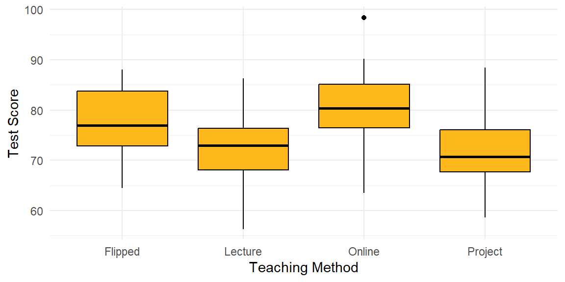
A school district tests four teaching methods—Lecture (A), Flipped Classroom (B), Project-Based (C), and Online (D)—on randomly assigned groups of students. After a six-week unit, each student takes the same standardized test. We want to know whether the average score differs across the four methods. Rather than perform six t-tests, we compute the ANOVA F statistic.
The boxplots hint at possible differences — the Online method appears to produce higher scores on average. To test this formally, we run the one-way ANOVA:
model <-aov(score ~ method, data = dat)summary(model)
            Df Sum Sq Mean Sq F value   Pr(>F)
method       3   1065   355.1   6.347 0.000674 ***
Residuals   76   4252    55.9
---
Signif. codes:  0 '***' 0.001 '**' 0.01 '*' 0.05 '.' 0.1 ' ' 1
Using \(\alpha=0.05\), the p-value is below 0.05, so we reject the null hypothesis. There is enough evidence to conclude that at least one teaching method produces a different mean score. We will identify which specific methods differ using Tukey’s HSD in the next section.
Recap
Keyword/Concept
Definition
One‑way ANOVA
A procedure for testing whether the means of three or more independent groups are equal.
Between‑group variability
Variability due to differences among group means.
Within‑group (error) variability
Variability of observations around their group means.
F statistic
The ratio \(\mathrm{MS}_{\mathrm{Between}}/\mathrm{MS}_{\mathrm{Error}}\) used to test \(H_0\) that all group means are equal.
Assumptions
Independence, normality of each group and equality of variances across groups.
Check your understanding
NoteProblems
Why is it not advisable to use multiple t‑tests to compare the means of four or more groups?
In your own words, explain what it means if the ANOVA F statistic is close to 1.
List the key assumptions of a one‑way ANOVA.
TipSolutions
Performing several independent t‑tests inflates the probability of making at least one Type I error (false positive). ANOVA tests all the means simultaneously and controls the overall error rate.
An F ratio near 1 means that the variability between group means is similar to the variability within groups. Under such circumstances the data are consistent with all groups having the same mean, and we would likely fail to reject \(H_0\).
The response variable should be continuous and approximately normally distributed in each group, observations should be independent, and the population variances should be equal.
13.2 Post‑hoc comparisons
“Statistics is a science in my opinion, and it is no more a branch of mathematics than are physics, chemistry, and economics; for if its methods fail the test of experience–not the test of logic–they will be discarded.” - John Tukey
The global F test in a one‑way ANOVA tells us that not all group means are equal, but it does not identify which pairs of means differ. Performing multiple two‑sample t‑tests on the same data inflates the family‑wise error rate. Post‑hoc procedures are designed to compare all pairs of group means while controlling the overall probability of making any false positives. The basic idea is to construct confidence intervals for each pair of means and adjust the critical values so that the chance of incorrectly claiming a difference remains at or below the chosen \(\alpha\) level.
Common post‑hoc methods
Several procedures exist for comparing means after an ANOVA. Here is a brief overview:
Fisher’s least significant difference (LSD) – performs unadjusted two‑sample t‑tests for each pair of means but only after the omnibus F test is significant. Simple to compute but does not control the family‑wise error rate when there are many comparisons.
Bonferroni – divides the desired significance level by the number of comparisons (or multiplies p‑values by that number). Valid for unequal sample sizes, but conservative when many comparisons are made.
Scheffé’s method – constructs simultaneous confidence intervals for all possible contrasts among means. Highly conservative but useful when testing complex hypotheses involving multiple groups.
Other specialized procedures include Holm’s sequential Bonferroni and Dunnett’s test (for comparing several treatments against a control), which we will not cover in detail here.
Tukey’s honestly significant difference (HSD)
Because it balances power and control of the family‑wise error rate, tukey’s hsd is the most widely used post‑hoc procedure in one‑way ANOVA. It relies on the studentized range distribution, which models the range of sample means standardized by the within‑group variability. After computing the ANOVA F test, the critical difference for comparing means of groups \(i\) and \(j\) is
\[
\mathrm{HSD} = \mathrm{q}_{1-\alpha, m, N - m}\,\sqrt{\frac{\mathrm{MS}_{\mathrm{Error}}}{2}\left(\frac{1}{n_i} + \frac{1}{n_j}\right)}
\]
where \(\mathrm{MS}_{\mathrm{Error}}\) is the within‑group mean square from the ANOVA table and \(\mathrm{q}_{1-\alpha, m, N - m}\) is the critical value from the studentized range distribution. For equal group sizes \(n_i = n_j = n\), this simplifies to \[
\mathrm{HSD} = \mathrm{q}\,\sqrt{\mathrm{MS}_{\mathrm{Error}}/n}
\]
A pair of sample means \(\bar{y}_{i\cdot}\) and \(\bar{y}_{j\cdot}\) is declared significantly different if \(|\bar{y}_{i\cdot} - \bar{y}_{j\cdot}| > \mathrm{HSD}\). Equivalently, the \(100(1-\alpha)\%\) confidence interval for the difference \(\bar{y}_{i\cdot} - \bar{y}_{j\cdot}\) is
Because Tukey’s method is based on the largest range among means, it controls the family‑wise error rate exactly when all group sizes are equal and remains robust for slight imbalances.
Performing Tukey’s HSD in R
After fitting the ANOVA with aov(), pass the model to TukeyHSD() to compute simultaneous confidence intervals for all pairwise differences:
model <-aov(score ~ method, data = dat)TukeyHSD(model)
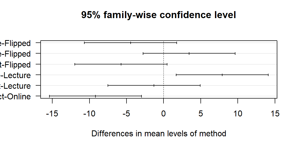
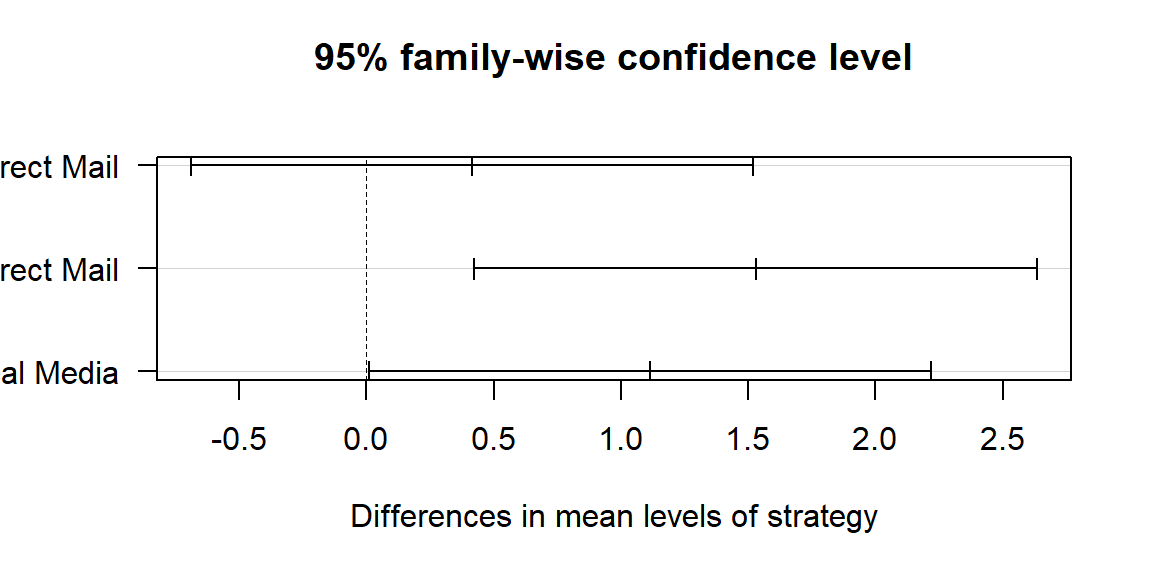
Each row shows the estimated difference in means between two groups, a 95% confidence interval, and an adjusted p-value. If the interval does not contain zero, the pair is significantly different at the family-wise level \(\alpha\). You can visualize all intervals at once with:
plot(TukeyHSD(model), las =1)
Always confirm the global F test is significant before interpreting post-hoc comparisons.
ExampleExample 13.2: Advertising strategy and weekly sales
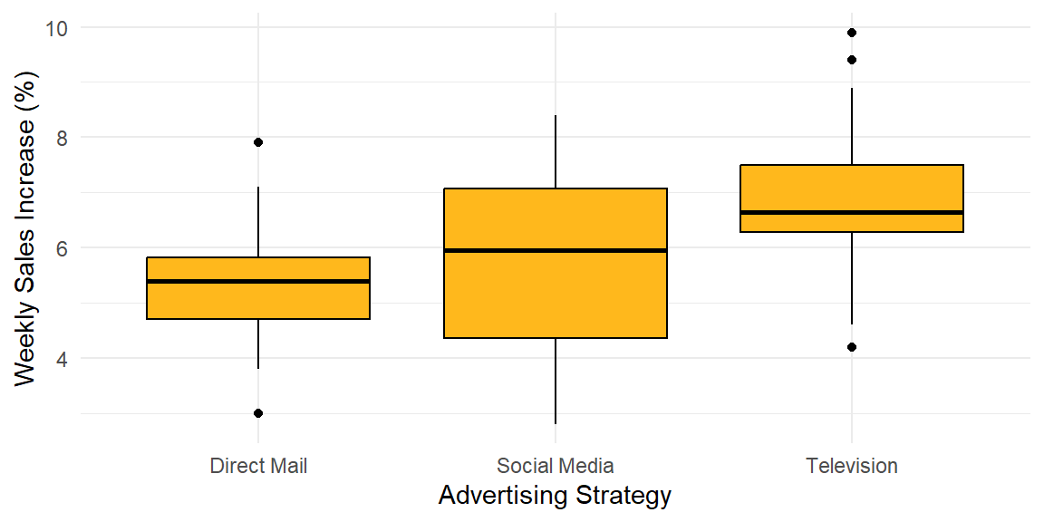
A retail company tests three advertising strategies - Social Media, Television, and Direct Mail - across 20 store regions each. The response variable is the percentage increase in weekly sales.
The one-way ANOVA tests whether the mean sales increase differs across strategies:
model2 <-aov(sales_increase ~ strategy, data = dat2)summary(model2)
            Df Sum Sq Mean Sq F value  Pr(>F)
strategy     2  25.04  12.521   5.932 0.00457 **
Residuals   57 120.31   2.111
---
Signif. codes:  0 '***' 0.001 '**' 0.01 '*' 0.05 '.' 0.1 ' ' 1
The F statistic is significant at \(\alpha=0.05\): there is enough evidence that at least one strategy produces a different mean sales increase. We apply Tukey’s HSD to identify which pairs differ:
TukeyHSD(model2)
  Tukey multiple comparisons of means
    95% family-wise confidence level

Fit: aov(formula = sales_increase ~ strategy, data = dat2)

$strategy
                          diff          lwr      upr     p adj
Social Media-Direct Mail 0.415 -0.690551852 1.520552 0.6404461
Television-Direct Mail   1.530  0.424448148 2.635552 0.0042906
Television-Social Media  1.115  0.009448148 2.220552 0.0476409
plot(TukeyHSD(model2), las =1)
The confidence interval for Television vs. Direct Mail does not include zero, indicating Television produces significantly higher sales increases than Direct Mail. Television also outperforms Social Media. The interval for Social Media vs. Direct Mail includes zero, so those two strategies are not significantly different from each other. In all three comparisons, we are 95% confident that the intervals contain the true pairwise differences.
Recap
Keyword/Concept
Definition
Post‑hoc test
A procedure for comparing pairs of group means after an ANOVA indicates that not all means are equal, while controlling the family‑wise error rate.
Tukey’s HSD
Uses the studentized range distribution to construct simultaneous confidence intervals for all pairwise differences; exact for equal group sizes and less conservative than Bonferroni.
Check your understanding
NoteProblems
In your own words, describe how Tukey’s HSD controls the family‑wise error rate.
TipSolutions
Tukey’s HSD uses the studentized range distribution to adjust the critical value. It accounts for the probability of the largest difference among group means exceeding a threshold, ensuring that the chance of falsely declaring any difference among the means is at most \(\alpha\).
13.3 Two‑way ANOVA and randomized blocks
“Statistics is the art of stating in precise terms that which one does not know.” - William Kruskal
When experiments involve two categorical factors—say, training program and experience level, or pricing tier and sales region—we can use a two‑way ANOVA. This model allows us to test for main effects of each factor and to examine whether the effect of one factor depends on the level of the other (the interaction). In certain designs where a second factor is used only to reduce variability and is not of substantive interest, we call it a randomized block design.
Model and hypotheses
Suppose we have two factors, \(A\) with \(a\) levels and \(B\) with \(b\) levels. Each treatment combination has \(n_{ij}\) observations. Let \(\mu_{ij}\) be the mean for combination \((i,j)\). We write the model as
where \(\mu\) is the grand mean, \(\alpha_i\) is the effect of level \(i\) of factor \(A\), \(\beta_j\) is the effect of level \(j\) of factor \(B\), \((\alpha\beta)_{ij}\) is the interaction effect, and \(\varepsilon_{ijk}\) are independent normal errors with common variance. The hypotheses for each effect are:
Main effect of \(A\):\[
H_0: \alpha_1 = \alpha_2 = \cdots = \alpha_a = 0\quad \text{vs.}\quad H_a: \text{At least one } \alpha_i \neq 0
\] This tests whether the mean response differs across levels of factor \(A\). This is equivalent to testing \[
H_0: \mu_1 = \mu_2 = \cdots = \mu_a\quad \text{vs.}\quad H_a: \text{At least one differs}
\] For all levels of factor \(B\).
Main effect of \(B\):\[
H_0: \beta_1 = \beta_2 = \cdots = \beta_b = 0\quad \text{vs.}\quad H_a: \text{At least one } \beta_j \neq 0
\] This is equivalent to testing \[
H_0: \mu_1 = \mu_2 = \cdots = \mu_b\quad \text{vs.}\quad H_a: \text{At least one differs}
\] for all levels of factor \(A\).
Interaction:\[
H_0: (\alpha\beta)_{ij} = 0\ \text{for all } i,j\quad \text{vs.}\quad H_a: \text{At least one } (\alpha\beta)_{ij} \neq 0
\] We can write this hypothesis without the math symbols as \[
\begin{align*}
&H_0: \text{There is no interaction between the two factors}\\
&H_a: \text{There is interaction between the two factors}
\end{align*}
\]
For each hypothesis, an F statistic is computed by dividing the mean square for that factor or interaction by the mean square error. Large F values suggest significant effects.
Partitioning variation
The two‑way ANOVA partitions the total variability into contributions from factor \(A\), factor \(B\), their interaction, and random error. For balanced designs with equal sample sizes \(n\) per combination, the sums of squares are
and the error sum of squares captures the variability of observations around their cell means. Dividing each sum of squares by its degrees of freedom yields mean squares for computing F statistics.
Randomized block designs
In a randomized block design, one factor is a blocking factor used to group similar experimental units and reduce variability. For example, in a sales study, representatives might be blocked by experience level; in an education study, classrooms might be blocked by school. The model is the same as the two‑way ANOVA model, but only the treatment factor is of interest; the block factor is included solely to account for variation among blocks.
We typically test the treatment effect and ignore the block effect. When the blocking factor is actually a repeated measurement on the same subject, we instead use a repeated measures ANOVA (see next section).
ExampleExample 13.3: Sales training programs and experience level
A company wants to study the effects of three sales training programs on employees at three different experience levels. There were 12 employees in each experience group who were then randomly assigned one of the three training programs. Each employee was rated on a sales performance score (0–100) after completing the program. The data are presented below:
0–2 years
3–5 years
6+ years
Program A
43, 43, 41, 42
53, 51, 53, 52
57, 55, 58, 56
Program B
52, 51, 51, 50
62, 61, 60, 61
65, 66, 66, 67
Program C
71, 72, 70, 71
81, 83, 82, 82
86, 84, 87, 86
In two-way ANOVA, a null hypothesis states that the population means are the same in each category of one factor, at each fixed level of the other factor.
For example, we could test \[
\begin{align*}
H_0: \text{Mean performance score is equal for all three programs for each experience level}
\end{align*}
\] We could also test \[
\begin{align*}
H_0: \text{Mean performance score is equal for all experience levels for each program}
\end{align*}
\]
Suppose the population means for each cell were as in table (a) below. Since the means are the same for all programs within each experience level, the first null hypothesis would be true. If the means were as in table (b), the means would be the same across experience levels within each program, so the second null hypothesis would hold.
(a)
Program
0–2 yr
3–5 yr
6+ yr
(b)
Program
0–2 yr
3–5 yr
6+ yr
Program A
60
70
80
Program A
50
50
50
Program B
60
70
80
Program B
60
60
60
Program C
60
70
80
Program C
70
70
70
Exploring Interaction Between Factors in Two-Way ANOVA
Investigating whether interaction occurs is important whenever we analyze multivariate relationships.
No interaction between two factors means that the effect of either factor on the response variable is the same at each category of the other factor.
We can enter the data and run the two-way ANOVA in R:
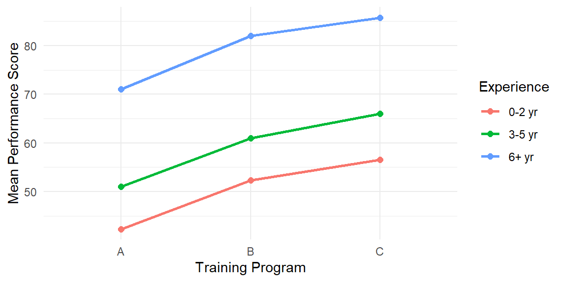
Approximately parallel lines indicate no interaction — the performance advantage of one program over another is consistent across experience levels.
At the 5% significance level, there is not enough evidence to conclude that there is interaction between Program and Experience Level. Because the interaction is not significant, we can test the main effects.
At the 5% significance level, there is enough evidence to conclude that at least one training program produces a different mean score for each experience level.
At the 5% significance level, there is enough evidence to conclude that at least one experience level produces a different mean score for each training program.
We can apply Tukey’s HSD to each main effect:
TukeyHSD(model3, which ="program")
  Tukey multiple comparisons of means
    95% family-wise confidence level

Fit: aov(formula = score ~ program * experience, data = dat3)

$program
         diff       lwr       upr p adj
B-A 10.333333  9.354468 11.312199     0
C-A 14.666667 13.687801 15.645532     0
C-B  4.333333  3.354468  5.312199     0
TukeyHSD(model3, which ="experience")
  Tukey multiple comparisons of means
    95% family-wise confidence level

Fit: aov(formula = score ~ program * experience, data = dat3)

$experience
               diff       lwr       upr p adj
3-5 yr-0-2 yr  9.00  8.021135  9.978865     0
6+ yr-0-2 yr  29.25 28.271135 30.228865     0
6+ yr-3-5 yr  20.25 19.271135 21.228865     0
Performing two‑way ANOVA in R
Use aov() with a model formula that includes both factors and their interaction (written as A * B, which expands to A + B + A:B). Pass the fitted model to summary() to obtain the ANOVA table.
model <-aov(response ~ factorA * factorB, data = dat)summary(model)
If you expect no interaction (e.g., a randomized block design), fit an additive model instead:
block_model <-aov(response ~ treatment + block, data = dat)summary(block_model)
To follow up with Tukey comparisons on the main effects:
TukeyHSD(model, which ="factorA")TukeyHSD(model, which ="factorB")
Recap
Keyword/Concept
Definition
Two‑way ANOVA
A model with two categorical explanatory variables (factors) that tests for main effects and interactions.
Main effect
The effect of a factor averaged over the levels of the other factor; tested by comparing \(\mathrm{MS}_{\text{factor}}\) to \(\mathrm{MS}_{\mathrm{Error}}\).
Interaction
Occurs when the effect of one factor depends on the level of the other; tested via an F ratio using \(\mathrm{MS}_{AB}\).
Randomized block design
A special two‑way ANOVA where one factor (the block) is used to control variability; only the treatment factor is of interest and the block factor accounts for nuisance variation.
Check your understanding
NoteProblems
Describe the difference between a main effect and an interaction effect in a two‑way ANOVA.
In a randomized block design with five treatments and four blocks, how many degrees of freedom are associated with the treatment, block and error sums of squares?
Why is it important to include the blocking factor in the model when analyzing a randomized block design?
TipSolutions
A main effect measures the average difference in the response across the levels of a factor, ignoring (averaging over) the other factor. An interaction effect tests whether the effect of one factor varies depending on the level of the other factor; if significant, the factors do not act independently.
The treatment factor has \(a-1\) degrees of freedom and the block factor has \(b-1\), where \(a\) is the number of treatments and \(b\) the number of blocks. The error degrees of freedom are \((a-1)(b-1)\) for a balanced design with one observation per cell. In this case, \(a=5\) and \(b=4\), so the treatment, block and error degrees of freedom are \(4\), \(3\) and \(12\), respectively.
The block factor captures variation among blocks. Omitting it would inflate the error term, reducing power to detect treatment differences. Including the blocking factor removes block‑to‑block variability from the error and improves precision.
13.4 Repeated measures ANOVA
“Beware of the problem of testing too many hypotheses; the more you torture the data, the more likely they are to confess, but confessions obtained under duress may not be admissible in the court of scientific opinion.” - Stephen Stigler
In many experiments the same experimental units are observed under multiple conditions—for example, recording a student’s quiz score at the beginning, middle, and end of a semester, or tracking an athlete’s performance across multiple training phases. Because measurements on the same subject are correlated, we cannot treat them as independent. A repeated measures ANOVA compares the means of three or more related measurements on the same subjects, taking into account this correlation.
Model and partitioning variance
For a one‑factor repeated measures design with \(m\) time points or conditions, we have \(n\) subjects each observed under all \(m\) conditions. Let \(y_{ij}\) denote the response of subject \(j\) at time \(i\). The model can be written as
where \(\mu\) is the grand mean, \(\tau_i\) is the effect of condition \(i\), \(s_j\) is the effect of subject \(j\) (a random subject effect), and \(\varepsilon_{ij}\) are error terms.
The ANOVA partitions the total variation into between‑treatments (conditions), between‑subjects, and error (within‑subjects) components. The F statistic for testing \(H_0: \tau_1=\cdots=\tau_m=0\) uses the mean square for treatments divided by the mean square error:
\[
F = \frac{\mathrm{MS}_{\text{Treatments}}}{\mathrm{MS}_{\text{Error}}}
\]
The error term is derived by subtracting the between‑subjects variation from the within‑subjects variation, leading to a smaller denominator and increased power compared with ordinary one‑way ANOVA.
Assumptions and sphericity
Repeated measures ANOVA requires that the differences between all pairs of conditions have equal variances—a property known as sphericity. If sphericity is violated (common when measurements are taken at closely spaced time points), the F statistics may be too liberal. Solutions include applying a Huynh–Feldt or Greenhouse–Geisser correction to the degrees of freedom or using a multivariate approach such as MANOVA. Another assumption is that the subjects are independent; repeated measures should not be confused with randomized block designs in which treatments are assigned to different units within a block.
ExampleExample 13.4: Student quiz scores over a semester
An instructor records quiz scores for 12 students at four points during the semester: Week 1, Week 5, Week 10, and Week 15. The goal is to determine whether mean quiz scores change over the course of the semester. The repeated measures ANOVA compares mean scores at the four time points.
At the 5% significance level, we test whether mean quiz scores differ across weeks. Tukey HSD confidence intervals for all pairwise week comparisons can then be examined to identify which weeks differ; intervals that do not include zero indicate a significant difference.
Conducting repeated measures ANOVA in R
Use aov() with an Error() term that specifies the subject and the within-subject factor:
model <-aov(response ~ time +Error(subject/time), data = dat)summary(model)
Here subject is a factor identifying each experimental unit and time is the repeated factor. To obtain Tukey comparisons, fit an ordinary two-way model (without the Error() wrapper) and pass it to TukeyHSD():
model_plain <-aov(response ~ time + subject, data = dat)TukeyHSD(model_plain, which ="time")
Recap
Keyword/Concept
Definition
Repeated measures ANOVA
A method for comparing means of three or more measurements on the same subjects, accounting for correlation among repeated observations.
Sphericity
The assumption that the variances of differences between all pairs of conditions are equal.
Between‑subjects variation
Variability due to differences among subjects; removed from the error term in repeated measures ANOVA to increase sensitivity.
Check your understanding
NoteProblems
Why can’t we treat repeated measurements on the same subject as independent observations?
What is the purpose of the sphericity assumption, and what adjustments can be made when it is violated?
Describe one advantage of the repeated measures design over a completely randomized design when the same subjects are measured multiple times.
TipSolutions
Measurements taken on the same subject are correlated; they share subject‑specific variability that violates the independence assumption of one‑way ANOVA. Repeated measures ANOVA models this correlation by separating between‑subjects and within‑subjects variation.
Sphericity ensures equal variances of pairwise differences between conditions. When sphericity is violated, F statistics can be adjusted using the Greenhouse–Geisser or Huynh–Feldt correction, or one can use a multivariate approach such as MANOVA.
Because each subject serves as their own control, repeated measures designs reduce the impact of between‑subject variability. This typically increases statistical power and requires fewer subjects to detect a given effect.