“There are some statistics that I’d like to share with you now, and they are numbers.” - Perd Hapley (Parks and Recreation)
With proper methods of gathering data, the values that a variable takes should arise from some random phenomenon. Even if the process is carefully controlled, chance still plays a role: different samples, repeated experiments, or repeated measurements rarely produce exactly the same result. Statistics exists precisely because of this randomness.
At first glance, the outcomes of random phenomena may seem naturally numerical. But this raises an interesting question:
Are outcomes themselves really numbers?
In reality, numbers are often just abstractions—labels we assign to describe and measure aspects of the world.
Consider weight. Weight is a physical force resulting from the interaction between mass and gravity. The force itself is not inherently a number; it is a physical property. We assign numbers—such as pounds or kilograms—to represent this property so that we can compare, analyze, and communicate it.
The same idea appears in many settings. Numerical values do not exist independently of measurement; rather, they are tools we use to represent outcomes.
Turning outcomes into numbers
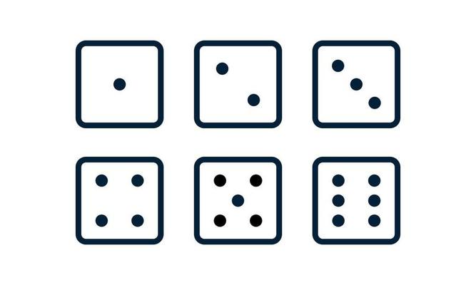
Think about rolling a six-sided die. Physically, the outcome is not really the number 1 or 6—it is a particular face landing upward.
By convention, we assign the labels
\[
\{1,2,3,4,5,6\}
\]
to these outcomes. We have created a rule that maps each physical outcome to a number.
Mathematically, this rule is a function whose:
domain is the sample space (all possible outcomes of the experiment), and
range is a subset of the real numbers.
This function is called a random variable.
A conceptual view of random variables
Another way to think about it is this:
When we talk about chance, we need a language that converts unpredictable events into something we can analyze mathematically. A random variable provides that language. It takes the messy details of “what happened” and translates them into a numerical value.
Importantly, the random variable is not the outcome itself; it is the rule that assigns numbers to outcomes.
For example, the outcome of tossing three coins might be (HHT), (TTT), or (HTH). A random variable could assign a number to each outcome, such as the number of heads observed.
Thus multiple different outcomes can produce the same numerical value.
Types of random variables
Random variables come in two broad types:
A discrete random variable has a countable set of possible values. These often arise from counting: number of successes, number of arrivals, number of defects, and so on.
A continuous random variable can take any value within an interval, such as height, temperature, or blood pressure. Continuous variables will be studied in more detail later; for now, our focus is primarily on discrete random variables.
Random variables describe processes, not data
A key idea is that a random variable describes the process that could generate data, not the data themselves. Before an experiment is conducted, the value of the random variable is unknown and may take many possible values.
Once the experiment occurs, we observe a realization (or observed value) of that random variable.
Examples
ExampleExample 6.1: Example from Medicine
Suppose a clinic screens 20 patients for a rare side effect of a new drug. Let
\[
X = \text{number of patients who experience the side effect}.
\]
Before screening begins, \(X\) could be any value from 0 to 20. Each possible value corresponds to many different combinations of patient outcomes. After the screening is complete, we observe one specific value (say \(x=3\)). This observed value is one realization of the random variable.1
Another clinic running the same experiment might observe a different value because the process contains randomness.
A loan officer at a regional bank reviews 10 small-business loan applications in a given week. Each application is independently evaluated and either approved or rejected based on the applicant’s creditworthiness. Let
\[
Y = \text{number of applications approved}.
\]
The possible values of \(Y\) are 0 through 10. Even before reviewing the applications, probability allows us to model how likely each outcome is based on the bank’s historical approval rate.
Why random variables matter
In both examples, the random variable converts a complex outcome—many individual successes or failures—into a single numerical summary. That number changes from trial to trial, but its behavior follows predictable probabilistic rules.
This abstraction is powerful. By representing outcomes numerically, we can:
describe variability mathematically,
calculate probabilities,
build models of uncertainty, and
make predictions about future observations.
In short, random variables are the bridge between real-world randomness and the mathematics of probability. They allow us to move from observing chance events to analyzing and understanding them quantitatively.
Recap
Keyword
Definition
random variable
A function that assigns a numeric value to each outcome of a random experiment.
Check your understanding
NoteProblems
Describe in your own words the difference between a random variable and the observed data.
Give an example of a discrete random variable in a medical context and list its possible values.
Is “blood type” (A, B, AB, O) a discrete random variable? Explain why or why not.
TipSolutions
The random variable is a rule that maps every possible outcome of a random experiment to a number. The observed data are the actual values of that mapping in one experiment. Before you flip 10 coins, the random variable “number of heads” could be 0–10; after you flip, you observe a single number, such as 4.
Let \(X\) be the number of patients out of 15 who respond favorably to a new therapy. The possible values of \(X\) are 0,1,2,…,15—one number for each possible count of responders.
Blood type is categorical rather than numeric. To analyze it as a random variable you would typically convert it to a binary indicator (e.g., 1 if type A, 0 otherwise). The categories A, B, AB and O do not have a numerical order, so blood type on its own is not a discrete random variable in the sense used here.
6.2 Probability Distributions and Their Properties
“Iacta alea est. (The die is cast.)” - Julius Ceasar
Once we have defined a discrete random variable, the next step is to describe how likely each of its possible values is. A probability distribution (also called a probability mass function) assigns a probability \(P(X=x)\) to every value \(x\) in the support of the random variable \(X\). A valid probability distribution must satisfy two simple but fundamental conditions:
Non‑negativity: For every possible value \(x\), the probability satisfies \(0 \le P(X=x) \le 1\). Probabilities can’t be negative or exceed one.
Sum to one: The probabilities of all possible outcomes add up to one: \[
\sum_{x} P(X=x) = 1\,.
\] This reflects the fact that something in the sample space must occur on each trial.
A probability distribution summarizes the long‑run behavior of a random variable. It tells you how often each value would appear if you repeated the experiment many times. Let’s look at an example.
ExampleExample 6.3: Items returned per online order
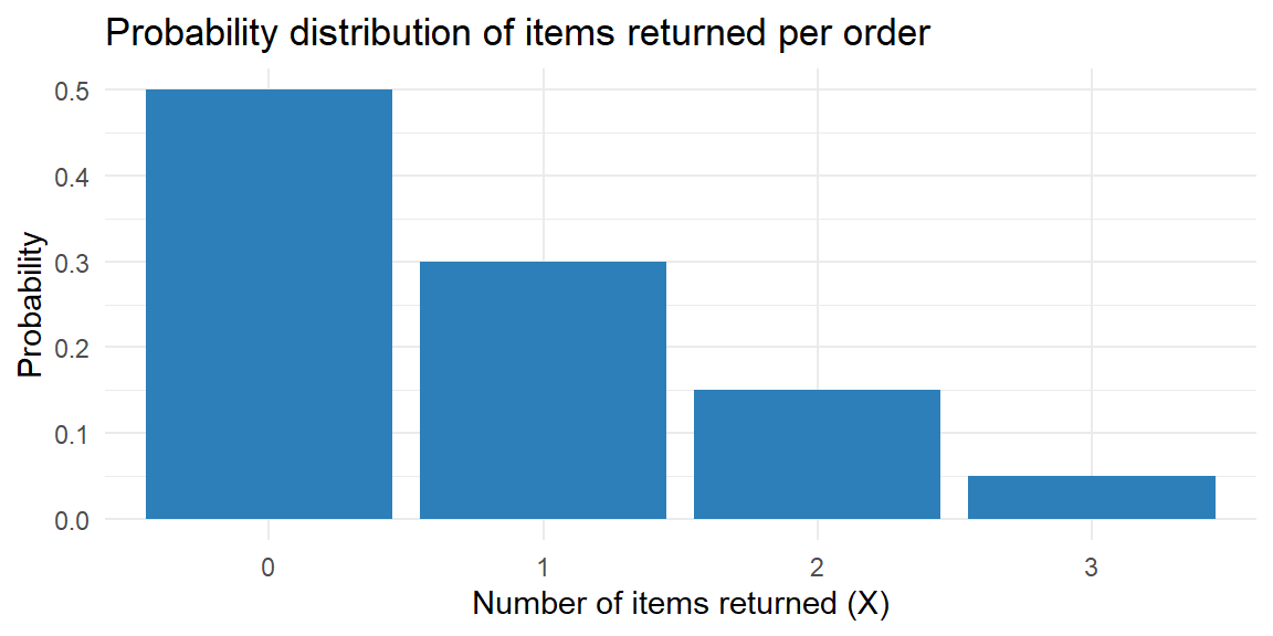
An online retailer tracks the number of items a customer returns per order. Based on company records, the random variable \(X\) = number of items returned per order takes the values 0, 1, 2, or 3 with the following probabilities:
\(x\)
0
1
2
3
\(P(X=x)\)
0.50
0.30
0.15
0.05
Every probability is between 0 and 1, and the probabilities sum to \[
0.50+0.30+0.15+0.05=1
\] Thus this table is a valid probability distribution. If a very large number of orders were examined, about 50% would have no returns, 30% would have one return, 15% two returns, and 5% three returns.
Commonly, the probability distribution of a discrete random variable is displayed with a bar chart. As long as the bar chart displays all possible values of the random variable and the probability of each value, it displays the probability distribution.
library(tidyverse)returns_dist <-tibble(returns =0:3,prob =c(0.50, 0.30, 0.15, 0.05))ggplot(returns_dist, aes(x =factor(returns), y = prob)) +geom_col(fill ="#2c7fb8") +labs(x ="Number of items returned (X)", y ="Probability",title ="Probability distribution of items returned per order") +theme_minimal()
ExampleExample 6.4: Defective products on an assembly line
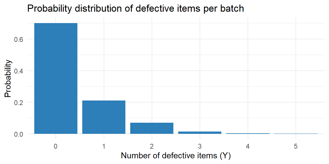
A quality control manager randomly samples batches of 5 products from an assembly line and records the number of defective items. The random variable \(Y\) = number of defective items per batch has the following probability distribution:
\(y\)
0
1
2
3
4
5
\(P(Y=y)\)
0.70
0.21
0.07
0.015
0.004
0.001
Each probability is between 0 and 1 and the probabilities sum to 1. Most batches (70%) contain no defects, but occasionally one or more defects occur.
library(tidyverse)defects_dist <-tibble(defects =0:5,prob =c(0.70, 0.21, 0.07, 0.015, 0.004, 0.001))ggplot(defects_dist, aes(x =factor(defects), y = prob)) +geom_col(fill ="#2c7fb8") +labs(x ="Number of defective items (Y)", y ="Probability",title ="Probability distribution of defective items per batch") +theme_minimal()
Validity checks
Sometimes you will be given a proposed distribution and asked whether it is valid. To check validity:
Make sure all probabilities are non‑negative and at most 1.
Add them up. If they sum to 1 (allowing for small rounding error) the distribution is valid; otherwise it is not.
If a distribution is not valid, you cannot use it until it is corrected or rescaled.
Recap
Keyword
Definition
probability distribution
A table, graph, or function assigning each possible value of a discrete random variable a probability between 0 and 1.
probability mass function (pmf)
Another name for the probability distribution of a discrete random variable.
Check your understanding
NoteProblems
Consider a random variable \(X\) that takes values 0, 1, 2 with \(P(X=0)=0.2\), \(P(X=1)=0.5\) and \(P(X=2)=0.4\). Is this a valid probability distribution? Explain.
A diagnostic test counts the number of positive samples among three blood samples from the same patient. Suggest a possible probability distribution for the number of positives and describe how you might visualize it.
The following table describes a proposed distribution for a random variable \(X\):
\(x\)
0
1
2
3
\(P(X=x)\)
0.3
\(–0.1\)
0.6
0.2
Is this distribution valid? Why or why not?
TipSolutions
The probabilities must sum to 1. Here \(0.2 + 0.5 + 0.4 = 1.1\), which is greater than 1, so this is not a valid distribution. One or more probabilities needs to be adjusted or rescaled.
The number of positive samples (\(Y\)) can be 0, 1, 2 or 3. A plausible distribution might be \(P(Y=0)=0.70\), \(P(Y=1)=0.20\), \(P(Y=2)=0.08\) and \(P(Y=3)=0.02\), but the actual numbers depend on the underlying infection probability. To visualize the distribution, enter these values and probabilities into R and create a bar chart with categories 0–3 on the X‑axis and probabilities on the Y‑axis.
A valid distribution cannot have negative probabilities. Because \(P(Z=1)=-0.1\) is negative, this table is invalid. You cannot assign negative weight to an outcome. The probabilities also sum to \(0.3-0.1+0.6+0.2=1.0\), but the negativity alone makes it invalid.
6.3 Mean and Standard Deviation of Discrete Distributions
“The most important questions of life are, for the most part, really only problems of probability.” -Pierre Simon, Marquis de Laplace
As stated previously in this course, we want to examine the center, spread, and shape when we have a data distribution. In Chapter 4, we discussed doing this with sample data where we calculate statistics like \(\bar{x}\), \(s\), and \(s^2\). These are sample statistics. The probability distribution tells us how likely each outcome of \(X\) is. Thus, we should view the probability distribution as a representation of the population.
We often want numeric values to describe the probability distribution in the same way we used statistics for the sample. Since these numeric values will be describing a population, these will be parameters.
It is common (but not always) to denote parameters with lowercase Greek letters. Below are some of the statistics we have discussed and the corresponding parameter.
Sample Statistic
Population Parameter
Mean
\(\bar{x}\)
\(\mu\)
Standard Deviation
\(s\)
\(\sigma\)
Variance
\(s^2\)
\(\sigma^2\)
The mean or expected value (denoted \(E(X)\)) of a discrete probability distribution is a weighted average: \[
\mu = E(X) = \sum_x x \cdot P(X=x)
\] You can think of the expected value as the long‑run average of \(X\) over many repetitions of the experiment.
ExampleExample 6.5: Florida lottery
The Florida Lottery runs two popular daily games called Pick 3 and Pick 4.
In Cash 3, players pay $1 to select three numbers in order, where each number ranges from 0 to 9. If the three numbers selected (e.g., 2–8–4) match exactly the order of the three numbers drawn, the player wins $500. The probability of winning Pick 3 is 0.001.
Play 4 is similar to Cash 3, but players must match four numbers (each number ranging from 0 to 9). For a $1 Play 4 ticket (e.g., 3–8–3–0), the player will win $5,000 if the numbers match the order of the four numbers drawn. The probability of winning Pick 4 is 0.0001
Let \(X\) be the random variable representing the amount of money you get for playing Pick 3.
The possible values of \(X\) is then
If you lose: \(-\$1\)
If you win: \(\$500-\$1=\$499\)
What is the expected amount of money you get for playing this game? \[
\begin{align*}
\mu &= \sum xP(X)\\\\
&{=-1(0.999)+499(0.001)}\\
&{=-0.999+.499}\\
&{=-0.5}
\end{align*}
\]
Let \(X\) be the random variable representing the amount of money you get for playing Pick 4.
The possible values of \(X\) is then
If you lose: \(-\$1\)
If you win: \(\$5000-\$1=\$4999\) The possible values of \(X\) is then
What is the expected amount of money you get for playing this game? \[
\begin{align*}
\mu &= \sum xP(X)\\\\
&{=-1(0.9999)+4999(0.0001)}\\
&{=-0.9999+.4999}\\
&{=-0.5}
\end{align*}
\]
ExampleExample 6.6: Life insurance
Suppose you work for an insurance company and you sell a $10,000 one-year term insurance policy at an annual premium of $290. Actuarial tables show that the probability of death during the next year for a person of your customer’s age, sex, health, etc., is .001. What is the expected gain (amount of money made by the company) for a policy of this type? \[X=\text{money made by the company per policy}\] If the customer lives: \(\$290\)
If the customer dies:\(\$290-\$10,000=-\$9710\)
The expected gain for a policy of this type: \[
\begin{align*}
\mu &= \sum xP(X)\\\\
&{=290(0.999)+(-9710)(0.001)}\\
&{=280}
\end{align*}
\]
Variance
The variance of \(X\), denoted \(\sigma^2\), measures how spread out \(X\) is around its mean. It is defined as \[
\begin{align*}
\sigma^2 = \sum_x (x - \mu)^2 P(X=x)
\end{align*}
\]
It weights squared deviations from the mean by the probability of each value. The standard deviation\(\sigma\) is simply the square root of the variance. It has the same units as \(X\) and describes the typical distance between \(X\) and its mean.
ExampleExample 6.7: Items returned per order revisited
Using the returns-per-order distribution from Example 6.3, we compute the mean and variance. Recall the probabilities:
On average, a customer returns 0.75 items per order. To compute the variance, we calculate \((x - \mu)^2\) for each \(x\):
\(x\)
\((x - 0.75)^2\)
\(P(X=x)\)
Contribution
0
\((0 - 0.75)^2 = 0.5625\)
0.50
\(0.5625 \times 0.50 = 0.28125\)
1
\((1 - 0.75)^2 = 0.0625\)
0.30
\(0.0625 \times 0.30 = 0.01875\)
2
\((2 - 0.75)^2 = 1.5625\)
0.15
\(1.5625 \times 0.15 = 0.234375\)
3
\((3 - 0.75)^2 = 5.0625\)
0.05
\(5.0625 \times 0.05 = 0.253125\)
The variance is the sum of the contributions: \[
\sigma^2 = 0.28125 + 0.01875 + 0.234375 + 0.253125 = 0.7875
\]
Thus the standard deviation is \[
\sigma = \sqrt{0.7875} \approx 0.887
\]
The typical number of returns per order deviates from the mean of 0.75 by about 0.89 items. Remember that the mean and standard deviation summarize the distribution; they do not need to correspond to actual observed values.
ExampleExample 6.8: Variance of the lottery and insurance examples
We now compute the variance and standard deviation for Examples 6.5 and 6.6 to understand the spread of each random variable alongside its expected value.
Florida Lottery — Pick 3
Recall that \(X\) = net gain per $1 ticket, with \(\mu_X = -0.50\).
The expected gain is $280 per policy, but the standard deviation of $316 illustrates why insurers must collect premiums from many policyholders: individual outcomes are highly variable, even when the average is predictable.
Recap
Keyword
Definition
expected value
Weighted average of a random variable: \(\sum_x x \,P(X=x)\). Another name for population mean.
Check your understanding
NoteProblems
A random variable \(W\) takes values 0, 1, 2, 3 with \(P(W=0)=0.1\), \(P(W=1)=0.2\), \(P(W=2)=0.4\) and \(P(W=3)=0.3\). Compute \(E(W)\) and \(\sigma_W\).
Explain in plain language what the standard deviation tells you about a random variable.
The standard deviation measures how far the values of a random variable typically fall from their average value. A small standard deviation means the values cluster tightly around the mean; a larger standard deviation means the values are more spread out and vary more from trial to trial.
6.4 The Binomial Distribution
“If people do not believe that mathematics is simple, it is only because they do not realize how complicated life is.” -John Louis von Neumann
Many count variables in medicine and biology arise from a simple process: you perform the same experiment \(n\) times, each time there are only two possible outcomes (success or failure), and the probability of success stays the same from trial to trial. The random variable that counts the number of successes in these \(n\) trials is said to follow a binomial distribution. We denote it by \(X \sim \mathrm{Bin}(n,p)\), where:
\(n\) is the number of independent trials.
\(p\) is the probability of success on each trial.
For the binomial model to be appropriate we must have:
A fixed number \(n\) of trials.
Each trial results in a success or failure.
The probability \(p\) of success is the same on every trial.
The trials are independent of each other.
Motivating Example
John Doe claims to possess extrasensory perception (ESP). An experiment is conducted in which a person in one room picks one of the integers 1, 2, 3, 4, 5 at random and concentrates on it for one minute. In another room, John Doe identifies the number he believes was picked. The experiment is done with three trials. After the third trial, the random numbers are compared with John Doe’s predictions. Doe got the correct result twice.
If John Doe does not actually have ESP and is merely guessing the number, what is the probability that he’d make a correct guess on two of the three trials?
Let \(X\) = number of correct guesses in \(n = 3\) trials. Then \(X = 0, 1, 2, \text{ or } 3\).
Let \(p\) denote the probability of a correct guess for a given trial.
If Doe is guessing, \(p = 0.2\) for Doe’s prediction of one of the five possible integers. Then, \(1 - p = 0.8\) is the probability of an incorrect prediction on a given trial.
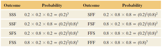
Denote the outcome on a given trial by \(S\) or \(F\), representing success or failure for whether Doe’s guess was correct or not. The table below shows the eight outcomes in the sample space for this experiment. For instance, \(FSS\) represents a correct guess on the second and third trials. It also shows their probabilities by using the multiplication rule for independent events.
The three ways John Doe could make two correct guesses in three trials are \(SSF\), \(SFS\), and \(FSS\). Each of these has probability equal to \[
(0.2)^2(0.8) = 0.032
\]
The total probability of two correct guesses (note these are mutually exclusive outcomes) is \[
\begin{align*}
P(SSF\cup SFS \cup FSS) = & (0.2)^2(0.8) + (0.2)^2(0.8) + (0.2)^2(0.8)\\
=& 3(0.2)^2(0.8)\\
=& 3(0.032)\\
=& 0.096
\end{align*}
\]
When the number of trials \(n\) is large, it’s tedious to write out all the possible outcomes in the sample space. But there’s a formula you can use to find binomial probabilities for any \(n\).
Probabilities for a Binomial Distribution
Denote the probability of success on a trial by \(p\). For \(n\) independent trials, the probability of \(x\) successes equals \[
P(X) = \binom{n}{x}p^x(1-p)^{n-x}, \qquad x=0, 1, 2, \ldots, n
\] where \[
\binom{n}{x}=\frac{n!}{x!(n-x)!}
\]
Let’s use this formula to find the probability that Doe would get only one correct in the previous section: \[
\begin{align*}
P(1) &= \frac{3!}{1!(3-1)!}0.2^1(1-0.2)^{3-1}\\\\
& {=\frac{6}{1}0.2(0.8)^2}\\
&{ =.3840}
\end{align*}
\]
Check to See If Binomial Conditions Apply
Before you use the binomial distribution, check that its three conditions apply. These are
binary data (success or failure),
the same probability of success for each trial (denoted by \(p\)), and
a fixed number \(n\) of independent trials.
One scenario where the assumptions do not apply is when sampling from a small population without replacement. When this occurs, the assumption of independence does not hold since the probability of success will change after each trial.
Guideline: Population and Sample Sizes to Use the Binomial For sampling \(n\) separate subjects from a population (that is, sampling without replacement), the exact probability distribution of the number of successes is too complex to discuss here, but the binomial distribution approximates it well when \(n\) is less than 10% of the population size. In practice, sample sizes are usually small compared to population sizes, and this guideline is satisfied.
Mean and Standard Deviation of the Binomial Distribution
Recall that the formula for the expected value of a discrete random variable is \[
E(X) = \mu = \sum xP(X)
\]
If we substitute in the binomial formula for \(P(X)\) in the formula for expected value we get[^2] \[
\begin{align*}
E(X) &= \mu = \sum_{x=0}^n x \frac{n!}{x!(n-x)!}p^x(1-p)^{n-x}\\
& {= np}
\end{align*}
\]
TipFor those who want to see the math:
\[
\begin{align*}
E[X]
&= \sum_{x=0}^{n} x \, P(X=x) \\
&= \sum_{x=0}^{n} x \binom{n}{x} p^{x}(1-p)^{\,n-x}.
\end{align*}
\]
So if we know the random variable is binomial, the expected value is just \(E(X) =np\).
The same thing can be done for the variance. If we know the random variable is binomial, the variance and standard deviation are \[
{\sigma^2=npq}\qquad\qquad{\sigma=\sqrt{npq}}
\]
TipFor those who want to see the math:
We begin from the probability mass function \[
P(X=x)=\binom{n}{x}p^x(1-p)^{,n-x}, \qquad x=0,1,\dots,n.
\]
Recall \[
\mathrm{Var}(X)=E[X^2]-(E[X])^2,
\] and from the previous result, \[
E[X]=np.
\]
Compute \(E[X(X-1)]\)
A useful identity is \[
X^2 = X(X-1)+X.
\] So we first compute \(E[X(X-1)]\).
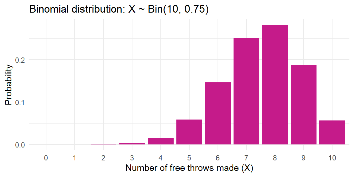
A professional basketball player makes free throws with probability 0.75. During a practice session, the player attempts 10 free throws. Let \(X \sim \mathrm{Bin}(10, 0.75)\) be the number of successful free throws. The probability of exactly \(x\) makes is \[
P(X = x) = \binom{10}{x} 0.75^x \, 0.25^{10 - x}.
\] For instance, the probability of making exactly 8 of 10 free throws is \[
\begin{align*}
P(X=8) &= \binom{10}{8} (0.75)^8 (0.25)^{2}\\
&= 45 \times 0.1001 \times 0.0625\\
&\approx 0.2816
\end{align*}
\] The expected number of makes is \[
E(X) = 10 \times 0.75 = 7.5
\] and the standard deviation is \[
\sigma = \sqrt{10 \times 0.75 \times 0.25} \approx 1.369
\]
A bar chart of the distribution shows that most of the probability mass is centered around 7 and 8:
ExampleExample 6.10: Voter support for a ballot measure
In a large city, 40% of registered voters support a proposed ballot measure to increase the public transit budget. A pollster randomly surveys 12 registered voters. Let \(Y \sim \mathrm{Bin}(12, 0.40)\) be the number of surveyed voters who support the measure.
The probability of exactly \(y\) supporters is \[
P(Y=y) = \binom{12}{y} 0.40^y \, 0.60^{12-y}.
\] The expected number of supporters is \(12 \times 0.40 = 4.8\) and the standard deviation is \(\sqrt{12 \times 0.40 \times 0.60} \approx 1.697\).
The probability of finding a majority (at least 7 of 12) in favor is \[
P(Y \ge 7) = 1 - P(Y \le 6) \approx 0.158
\] meaning there is roughly a 16% chance that a random sample of 12 voters would show a majority in support, even though the true support level is 40%.
ExampleExample 6.11: Passing a standardized exam
A state standardized exam has a historical pass rate of 70%. A school administrator randomly selects 6 student score reports to review. Let \(X \sim \mathrm{Bin}(6, 0.70)\) be the number of students who passed. The full probability distribution is:
\(x\)
0
1
2
3
4
5
6
\(P(X=x)\)
0.001
0.010
0.060
0.185
0.324
0.303
0.118
The expected number of passing students is \(E(X) = 6 \times 0.70 = 4.2\) and the standard deviation is \(\sigma = \sqrt{6 \times 0.70 \times 0.30} \approx 1.122\).
Computing Binomial Probabilities in R
R provides four built-in functions for working with the binomial distribution. Each function name follows the convention [prefix]binom, where the prefix determines what is computed:
Function
What it computes
dbinom(x, size, prob)
\(P(X = x)\) — the exact probability of \(x\) successes
pbinom(q, size, prob)
\(P(X \le q)\) — the cumulative probability up to \(q\)
qbinom(p, size, prob)
The smallest \(x\) such that \(P(X \le x) \ge p\) (the quantile function)
rbinom(n, size, prob)
Generates \(n\) random draws from \(\mathrm{Bin}(\texttt{size}, \texttt{prob})\)
The size argument is the number of trials and prob is the probability of success on each trial.
The code below reproduces the key probabilities from the examples in this section.
# Motivating example: ESP guessing (n = 3, p = 0.2)# P(X = 2) -- probability Doe guesses correctly exactly twicedbinom(2, size =3, prob =0.2)
[1] 0.096
# P(X = 1) -- probability of exactly one correct guessdbinom(1, size =3, prob =0.2)
You can also simulate binomial data with rbinom(). For example, to simulate the free throw scenario 10,000 times and compare the simulated proportions to the theoretical probabilities:
The distribution of the number of successes in \(n\) independent trials with success probability \(p\).
binomial pmf
\(P(X=x) = \binom{n}{x} p^x (1-p)^{n-x}\) for \(x=0,\dots,n\).
Check your understanding
NoteProblems
An antibiotic cures a bacterial infection in 75 % of cases. In a study of 8 independent patients, let \(X\) be the number of patients cured. Compute:
\(P(X=6)\).
\(P(X\le 4)\).
\(E(X)\) and \(\sigma\)
A gene occurs in 15% of the population. You sample 10 individuals at random. What is the probability that exactly 2 individuals carry the gene? What is the probability that at least one individual carries the gene?
A researcher flips a biased coin (probability of heads is 0.6) 5 times. Does the number of heads follow a binomial distribution? Why or why not?
Describe a real‑world scenario where the binomial model would not be appropriate even though the outcome is a count of successes. Explain which assumption is violated.
TipSolutions
Here \(X \sim \mathrm{Bin}(n=8,p=0.75)\). a) \(P(X=6) = \binom{8}{6} 0.75^6 0.25^2 = 28 \times 0.1779785 \times 0.0625 \approx 0.311\). b) \(P(X\le 4) = \sum_{x=0}^4 \binom{8}{x} 0.75^x 0.25^{8-x} \approx 0.0081\) (you can compute this with a calculator or software). c) The mean is \(E\)X\(=8\times 0.75=6\) and the standard deviation is \(\sigma_X=\sqrt{8\times 0.75 \times 0.25}=\sqrt{1.5}\approx 1.225\).
Let \(Y \sim \mathrm{Bin}(10,0.15)\). Then \(P(Y=2) = \binom{10}{2} (0.15)^2 (0.85)^8 \approx 45 \times 0.0225 \times 0.27249 \approx 0.276\). The probability of at least one carrier is \(1 - P(Y=0) = 1 - 0.85^{10} \approx 1 - 0.1969 = 0.8031\).
Yes. Each flip is a trial with two outcomes (heads or tails), the probability of heads is the same (0.6) on each flip, and the flips are assumed independent. Therefore the number of heads in 5 flips follows \(\mathrm{Bin}(5,0.6)\).
Suppose we sample 10 patients from a small village where tuberculosis is contagious and individuals tend to be exposed through one another. Let \(X\) be the number of infected patients. Even if each individual infection has some probability \(p\), the infections are not independent: once one person is infected, the chance that their neighbor is infected rises. This dependence violates the independent‑trials assumption of the binomial model, so \(X\) would not follow a binomial distribution.
Note that we use a uppercase letter to denote the random variable itself. We use a lowercase letter when denoting a realization of that random variable.↩︎