“I try not to get involved in the business of prediction. It’s a quick way to look like an idiot.” - Warren Ellis
6.1 Using the Model for Estimation and Prediction
Now that we have fit the model \[
y = {\beta}_0 + {\beta}_1 x + \varepsilon
\] and assessed how good of fit the model is, we can now use the model estimation and prediction.
Recall that the mean of \(y_{i}\) for some value of \(x_{i}\) is the population line \(\beta_{0}+\beta_{1}x_{i}\) evaluated at \(x_{i}\).
So we can estimate the mean of \(y_{i}\) for some value of \(x_{i}\) by evaluating the model estimated with the least squares estimators: \[\begin{align*}
\hat{y}_{i} & =b_0+b_1x_{i}
\end{align*}\]
We say \(\hat{y}_{i}\) is a point estimator for the population mean \(\beta_{0}+\beta_{1}x_{i}\).
6.1.1 The Sampling Distribution of \(\hat{y}\)
We will want to make an inference for the population mean response at some value of the predictor variable \(x_{i}\).
We have a point estimator \(\hat{y}_{i}\). We will now examine the sampling distribution of \(\hat{y}_{i}\) and use it to make a confidence interval for the mean response \(\beta_{0}+\beta_{1}x_{i}\).
6.1.2 Linear Combination of \(y\)
We will denote the value of \(x\) at which we want to estimate the mean response as \(x_{h}\). So the value of \(y\) at \(x_{h}\) will be \(y_{h}\)
We write \(\hat{y}_{h}\) as \[\begin{align*}
\hat{y}_{h} & =\underbrace{b_0}_{(3.2)}+\underbrace{b_1}_{(3.1)}x_{h}\\
& =\sum c_{i}y_{i}+\sum k_{i}y_{h}x_{h}\\
& =\sum\left(c_{i}+k_{i}x_{h}\right)y_{h}
\end{align*}\]
Thus, \(\hat{y}_{j}\) is a linear combination of the observed \(y_{i}\) which are normally distributed. Then by Theorem 4.2, \(\hat{y}_{j}\) is normally distributed.
6.1.3 The Mean of \(\hat{y}_h\)
Using Theorem 4.2, we have the mean as \[\begin{align*}
\sum\left(c_{i}+k_{i}x_{h}\right)E\left[y_{h}\right] & =\left(\underbrace{\sum c_{i}}_{=1}+x_{h}\underbrace{\sum k_{i}}_{=0}\right)\left(\beta_{0}+\beta_{1}x_{h}\right)\\
& =\beta_{0}+\beta_{1}x_{h}
\end{align*}\]
6.1.4 The Variance of \(\hat{y}_h\)
Using Theorem 4.3, we have the variance as \[\begin{align*}
Var\left[\hat{y}_{h}\right] & =\sigma^{2}\left(\frac{1}{n}+\frac{\left(x_{h}-\bar{x}\right)^{2}}{\sum\left(x_{i}-\bar{x}\right)^{2}}\right)
\end{align*}\]
So the sampling distribution of \(\hat{y}_{h}\) is \[
\begin{align}
\hat{y}_{h} & \sim N\left(\beta_{0}+\beta_{1}x_{h},\sigma^{2}\left(\frac{1}{n}+\frac{\left(x_{h}-\bar{x}\right)^{2}}{\sum\left(x_{i}-\bar{x}\right)^{2}}\right)\right)
\end{align}
\tag{6.1}\]
We will need to estimate \(\sigma^{2}\) with \(s^{2}\). This will mean that the confidence interval is a \(t\) interval.
6.1.5 Confidence Interval for the Mean Response
A \(\left(100-\alpha\right)100\%\) confidence interval for the mean response is \[
\begin{align}
\hat{y}_{h} \pm t_{\alpha/2}\sqrt{s^{2}\left(\frac{1}{n}+\frac{\left(x_{h}-\bar{x}\right)^{2}}{\sum\left(x_{i}-\bar{x}\right)^{2}}\right)}
\end{align}
\tag{6.2}\]
6.2 Predicting the Response
6.2.1 The Predicted Response
Previously, we estimated the mean of all \(y\)s for some value of \(x_{h}\).
Suppose we want to predict one value of the response variable \(y\) for some value of \(x_{h}\). We will denote this predicted value as \(y_{h\left(pred\right)}\).
6.2.2 Prediction When the True Line is Known
Our best point predictor will be the mean (since it is the most likely value). If we knew the the true regression line, then we could predict at \[\begin{align*}
y_{h\left(pred\right)} & =\beta_{0}+\beta_{1}x_{h}
\end{align*}\]
The variance of \(y_{h\left(pred\right)}\) would be \[\begin{align*}
Var\left[y_{h}\right] & =\sigma^{2}
\end{align*}\]
Then we can be \(\left(1-\alpha\right)100\%\) confident that the predicted value \(y_{h\left(pred\right)}\) is \[\begin{align*}
z_{\alpha/2}\sigma
\end{align*}\] units away from the line.
If we don’t know \(\sigma\), then we could estimate it with \(s\) and we can be \(\left(1-\alpha\right)100\%\) confident that the predicted value \(y_{h\left(pred\right)}\) is \[\begin{align*}
t_{\alpha/2}s
\end{align*}\] units away from the line.
6.2.3 Predicting When the True Line is Unknown
Of course, we do not know the true regression line. We will need to estimate it first.
Using the least squares estimators, we will predict at \[\begin{align*}
\hat{y}_{h} & =b_0+b_1x_{h}
\end{align*}\]
6.2.4 The Variance of the Predicted Response
Since \(\hat{y}_{h}\) is a random variable, it will have a sampling distribution. From Equation 6.1, that sampling distribution has a variance of \[\begin{align*}
Var\left[\hat{y}_{h}\right] & =\sigma^{2}\left(\frac{1}{n}+\frac{\left(x_{h}-\bar{x}\right)^{2}}{\sum\left(x_{i}-\bar{x}\right)^{2}}\right)
\end{align*}\]
Thus, the variance of the prediction of \(y_{h\left(pred\right)}\) will be the sum of the variance of the response variable: \[\begin{align*}
\sigma^{2}
\end{align*}\] and the variance of the fitted line: \[\begin{align*}
\sigma^{2}\left(\frac{1}{n}+\frac{\left(x_{h}-\bar{x}\right)^{2}}{\sum\left(x_{i}-\bar{x}\right)^{2}}\right)
\end{align*}\]
So the variance of \(y_{h\left(pred\right)}\) is \[\begin{align*}
Var\left[y_{h\left(pred\right)}\right] & =\sigma^{2}+\sigma^{2}\left(\frac{1}{n}+\frac{\left(x_{h}-\bar{x}\right)^{2}}{\sum\left(x_{i}-\bar{x}\right)^{2}}\right)\\
& =\sigma^{2}\left(1+\frac{1}{n}+\frac{\left(x_{h}-\bar{x}\right)^{2}}{\sum\left(x_{i}-\bar{x}\right)^{2}}\right)
\end{align*}\]
Since \(y\) is normally distributed, then we have a \(\left(100-\alpha\right)100\%\) prediction interval for \(y_{h\left(pred\right)}\) as \[
\begin{align}
{\hat{y}_{h} \pm t_{\alpha/2}\sqrt{s^{2}\left(1+\frac{1}{n}+\frac{\left(x_{h}-\bar{x}\right)^{2}}{\sum\left(x_{i}-\bar{x}\right)^{2}}\right)}}
\end{align}
\]#eq-w2_21
To find the confidence and prediction intervals, we must construct a new data frame with the value of \(X_h\). This value is then used, along with the lm object, to the predict function. If no value of \(X_h\) is provided, then predict will provide intervals for all values of \(x\) found in the data used in lm.
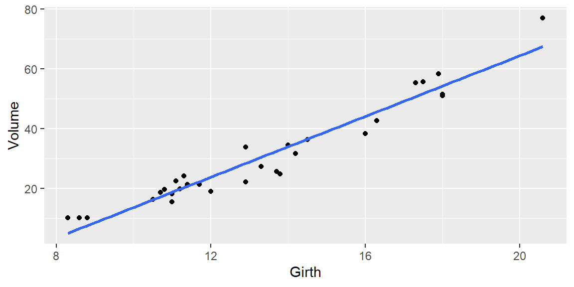
Recall the least squares fit:
# get a 95% confidence interval for the mean Volume# when girth is 16xh=data.frame(Girth=16)fit |>predict(xh,interval="confidence",level=0.95)
       fit      lwr      upr
1 44.11024 42.01796 46.20252
# 95% prediction interval for one value of Volume when# girth is 16fit |>predict(xh,interval="prediction",level=0.95)
       fit     lwr      upr
1 44.11024 35.1658 53.05469
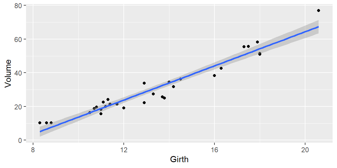
We can plot the confidence interval for all values of \(x\) by using the geom_smooth command in ggplot:
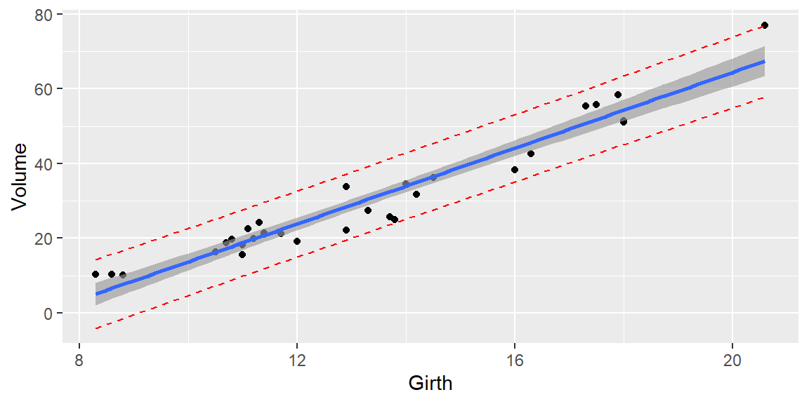
We can plot prediction intervals by adding them manually:
pred_int = fit |>predict(interval="prediction",level=0.95) |>as.data.frame()dat =cbind(trees, pred_int)ggplot(data=dat, aes(x=Girth, y=Volume)) +geom_point() +geom_smooth(method='lm',formula=y~x) +geom_line(aes(y=lwr), color ="red", linetype ="dashed") +geom_line(aes(y=upr), color ="red", linetype ="dashed") +geom_smooth(method=lm, se=TRUE)
Note that the prediction interval (the red dashed lines) is wider than the prediction interval. This is because the prediction interval has the extra source of variability.
6.2.5 Extrapolation and Precision
When using the least squares prediction equation to estimate the mean value of \(y\) or to predict a particular value of \(y\) for values of \(x\) outside the range of your sample data, you may encounter much larger errors than expected. This practice is known as extrapolation.
Even though the least squares model might fit the data well within the range of sample \(x\) values, it can poorly represent the true model for values of \(x\) outside this range.
As the sample size \(n\) increases, the width of the confidence interval decreases. In theory, you can achieve as precise an estimate of the mean value of \(y\) as desired for any given \(x\) by selecting a large enough sample.
Similarly, the prediction interval for a new value of \(y\) also becomes narrower as \(n\) increases. However, the prediction interval has a lower limit, which is reflected in the formula:
\[
\hat{y} \pm z_{\alpha/2} \sigma
\]
This means that no matter how large the sample, the interval can’t shrink below a certain size unless you reduce the standard deviation of the regression model, \(\sigma\). To make more accurate predictions for new values of \(y\), you must improve the model—either by using a curvilinear relationship with \(x\), adding new independent variables, or both.