25Multinomial Logistic Regression and Poisson Regression
“It’s easy to lie with statistics; it is easier to lie without them.” - Frederick Mosteller
25.1 Nominal Response
Logistic regression is most frequently used to model the relationship between a dichotomous response variable and a set of predictor variables.
On occasion, however. the response variable may have more than two levels.
Logistic regression can still be employed by means of a polytomous-or multinomial-logistic regression model.
Multinomial logistic regression models are used in many fields. In business, for instance, a market researcher may wish to relate a consumer’s choice of product (product A, product B. product C) to the consumer’s age, gender, geographic location and several other potential explanatory variables.
This is an example of nominal multinomial regression because the response categories are purely qualitative and not ordered in any way.
Ordinal response categories can also be modeled using multinomial regression.
For example, the relation between severity of disease measured on an ordinal scale (mild, moderate, severe) and age of patient, gender of patient, and some other explanatory variables may be of interest.
The response variable \(y\) must be coded in the same way as indicator variables except we will need an indicator variable for each category of \(y\).
Instead of going through the details, we will illustrate with tidymodels.
Example
A study was undertaken to determine the strength of association between several risk factors and the duration of pregnancies.
The risk factors considered were mother’s age, nutritional status, history of tobacco use, and history of alcohol use.
The response of interest, pregnancy duration, is a three-category variable that was coded as follows: \[
\begin{align*}
y_{i} &\quad \textbf{Pregnancy Duration Category}\\
1 &\quad \text{Preterm (less than 36 weeks)}\\
2 &\quad \text{Intermediate term (36 to 37 weeks)}\\
3 &\quad \text{Full term (38 weeks or greater)}
\end{align*}
\]
Relevant data for 102 women who had recently given birth at a large metropolitan hospital were obtained.
X variables include:
Nutritional status (\(x_1\)), is an index of nutritional status (higher score denotes better nutritional status).
Age was categorized into three groups. It is represented by two indicator variables (\(x_2\) and \(x_3\)): \[
\begin{align*}
x_{2} &\quad x_{3} & \textbf{Class}\\
1 &\quad 0 & \text{Less than or equal to 20}\\
0 &\quad 0 & \text{21 to 30}\\
0 &\quad 1 & \text{Greater than 30}
\end{align*}
\]
Alcohol (\(x_4\)) and smoking history (\(x_5\)) were also qualitative predictors; the categories were “Yes” (coded 1) and “No” (coded 0).
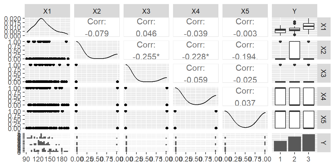
Let’s read in the data and visualize the variables.
Note in the summary, we have two regression fits. What we actually have done is model the odds of the probability of being in category 2 to the probability of being in category 1.
We also modeled the odds of the probability of being in category 3 to the probability of being in category 1.
So we call category 1 the baseline category.
To get the effect on the odds ratio for each coefficient:
We can compare the predicted classes versus the observed classes.
table(preds_class, dat$Y)
preds_class  1  2  3
          1 13  5  4
          2  8 23  5
          3  4  7 32
25.2 Ordinal Regression
25.2.1 Ordinal Response
When the response variable \(Y\) takes on categorical responses that can be put into order, then the multinomial logistic regression can still be used.
However, a more effective strategy, yielding a more parsimonious and more easily interpreted model, results if the ordering of the categories is taken into account explicitly.
The model that is usually employed is called the proportionalodds model
The proportional odds model for ordinal logistic regression models the cumulative probabilities \[
P(y_i\le j)
\] rather than the specific category probabilities \[
P(y_i=j)
\] as was the case for nominal logistic regression.
Again, we will skip the details and illustrate with R using the pregnancy data from the last section.
We consider now another nonlinear regression model where the response outcomes are discrete.
Poisson regression is useful when the outcome is a count, with large-count outcomes being rare events.
For instance, the number of times a household shops at a particular supermarket in a week is a count, with a large number of shopping trips to the store during the week being a rare event. A researcher may wish to study the relation between a family’s number of shopping trips to the store during a particular week and the family’s income, number of children, distance from the store, and some other explanatory variables.
As another example, the relation between the number of hospitalizations of a member of a health maintenance organization during the past year and the member’s age, income, and previous health status may be of interest.
The Poisson distribution can be utilized for outcomes that are counts (\(y_i = 0, 1,2, ...\) ), with a large count or frequency being a rare event.
25.3.1 The Poisson Distribution
The Poisson probability distribution is \[
f(Y) = \frac{\mu^Y \exp(-\mu)}{Y!}
\]
The mean and variance of a Poisson distribution are \[
\begin{align*}
E\{Y\} &= \mu\\
\sigma^2\{Y\} &=\mu
\end{align*}
\]
Note that the variance is the same as the mean.
Hence, if the number of store trips follows the Poisson distribution and the mean number of store trips for a family with three children is larger than the mean number of trips for a family with no children, the variances of the distributions of outcomes for the two families will also differ.
25.3.2 Poisson Regression
We start with the regression model \[
\begin{align*}
y_{i} & =E\left[ y_{i}\right] +\varepsilon_{i}\qquad i=1,2,\ldots,n
\end{align*}
\]
The mean response for the \(i\)th case, to be denoted now my \(\mu_{i}\) for simplicity, is assumed as always to be a function of the set of predictor variables \(x_{1},\ldots,x_{p-1}\).
We use the notation \(\mu\left(\textbf{X}_{i},\boldsymbol{\beta}\right)\) to denote the function that relates the mean response \(\mu_{i}\) to \(\textbf{X}_{i}\), the values of the predictor variables for case \(i\), and \(\boldsymbol{\beta}\), the values of the regression coefficients.
Some commonly used functions for Poisson regression are \[
\begin{align*}
\mu_{i}= & \mu\left(\textbf{X}_{i},\boldsymbol{\beta}\right)=\textbf{X}_{i}^{\prime}\boldsymbol{\beta}\\
\mu_{i}= & \mu\left(\textbf{X}_{i},\boldsymbol{\beta}\right)=\exp\left(\textbf{X}_{i}^{\prime}\boldsymbol{\beta}\right)\\
\mu_{i}= & \mu\left(\textbf{X}_{i},\boldsymbol{\beta}\right)=\ln\left(\textbf{X}_{i}^{\prime}\boldsymbol{\beta}\right)
\end{align*}
\]
In all three cases, the mean response \(\mu_{i}\) must be nonnegative.
Since the distribution of the error terms \(\varepsilon_{i}\) for Poisson regression is a function of the distribution of the response \(y_{i}\), which is Poisson, it is easiest to state the Poisson regression model in the following form:
\(y_{i}\) are independent Poisson random variables with expected values \(\mu_{i}\) where \[
\begin{align*}
\mu_{i} & =\mu\left(\textbf{X}_{i},\boldsymbol{\beta}\right)
\end{align*}
\]
The most commonly used response function is \(\mu_{i}=\exp\left(\textbf{X}_{i}^{\prime}\boldsymbol{\beta}\right)\).
Example
The Miller Lumber Company is a large retailer of lumber and paint, as well as of plumbing, electrical, and other household supplies.
During a representative two-week period, in-store surveys were conducted and addresses of customers were obtained. The addresses were then used to identify the metropolitan area census tracts in which the customers reside.
At the end of the survey period, the total number of customers who visited the store from each census tract within a 10-mile radius was determined and relevant demographic information for each tract (average income, number of housing units, etc.) was obtained.
Several other variables expected to be related to customer counts were constructed from maps, including distance from census tract to nearest competitor and distance to store.
Initial screening of the potential predictor variables was conducted which led to the retention of five predictor variables:
\(x_1\): Number of housing units
\(x_2\): Average income, in dollars
\(x_3\): Average housing unit age, in years
\(x_4\) : Distance to nearest competitor, in miles
\(x_5\): Distance to store, in miles
\(y_i\) : Number of customers who visited store from census tract