“All generalizations are false, including this one.” - Mark Twain
19.1 Ridge Regression
We have seen that multicollinearity causes the least squares estimates to be imprecise.
If we allow some bias in our estimators, then we can have estimators that are more precise. This is due to the relationship \[
\begin{align*}
E\left[\left(\hat{\beta}-\beta\right)^{2}\right] & =Var\left[\hat{\beta}\right]+\left(E\left[\hat{\beta}\right]-\beta\right)^{2}
\end{align*}
\]
Ridge regression starts by transforming the variables as \[
\begin{align}
Y_{i}^{*} & =\frac{1}{\sqrt{n-1}}\left(\frac{Y_{i}-\overline{Y}}{s_{Y}}\right)\nonumber\\
X_{ik}^{*} & =\frac{1}{\sqrt{n-1}}\left(\frac{X_{ik}-\overline{X}_{k}}{s_{k}}\right)\label{eq:w5_23}
\end{align}
\] This is known as the correlationtransformation.
The estimates are then found by penalizing the least squares criterion \[
\begin{align}
Q & =\sum\left[Y_{i}^{*}-\left(b_{1}^{*}X_{i1}^{*}+\cdots+b_{p-1}^{*}X_{i,p-1}^{*}\right)\right]^{2}+\lambda\left[\sum_{j=1}^{p-1}\left(b_{j}^{*}\right)^{2}\right]
\end{align}
\tag{19.1}\]
The added term gives a penalty for large coefficients. Thus, the estimators are biased toward 0. Because of this, the ridge estimators are called shrinkage estimators.
There are a number of methods for determining \(\lambda\) which are beyond the scope of our class. In R, we will use the glmnet engine to fit the model.
The ridge estimators are more stable than the ols estimators, however, the distributional properties of these estimators are not easily found.
Example 19.1 (Ridge Regression for mtcars) Let’s examine the mtcars data last seen in Example 16.3. Recall that disp, hp, and wt need to be log-transformed to make the relationships linear.
We will now use the “glmnet” engine for ridge regression. We set the value of \(\lambda\) in Equation 19.1 with the penalty argument in linear_reg. We will just arbitrarily use 0.1 for now. We will later in this section discuss how to choose a value of penalty.
We see that log_wt has the biggest impact on mpg since it has the largest coefficient in magnitude. The negative sign just indicates that the linear relationship between log_wt and mpg is negative.
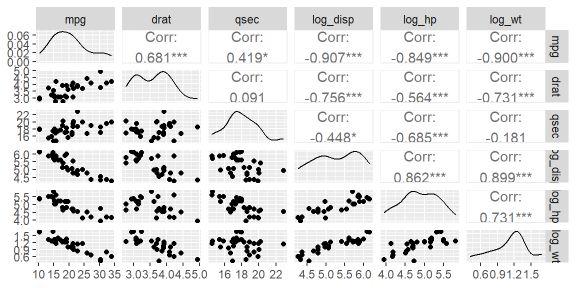
We also see that drat has the smallest impact on mpg given the other variables are in the model, followed by qsec for the second smallest impact. Let’s reexamine the scatterplot matrix to see if this make sense.
Looking at the plots of mpg versus the other variables, we see that a linear relationship is apparent for all of the predictors. Between drat and qsec, drat appears stronger (\(r=0.681\)) than qsec (\(r=0.419\)). But why did ridge regression show us that qsec has a larger impact on mpg than drat? Ridge regression shows the impact given the other variables are included in the model. Looking at the scatterplot matrix, drat is more correlated with the other predictor variables than qsec. Thus, when every other predictor is included, drat does not explain much more variability in mpg. Thus, it is not as important.
19.1.1 The effect of the penalty
In Example 19.1, we chose the penalty (\(\lambda\)) arbitrarily to be 0.1. Are there other values of penalty that would fit the data better?
We can try different penalties using the tidy function:
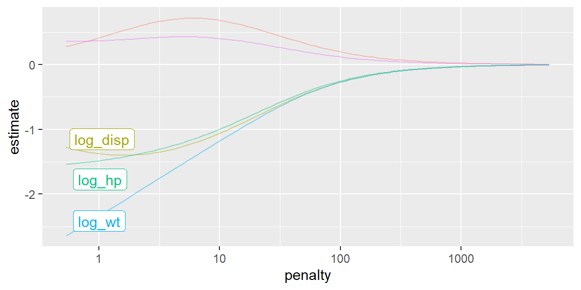
We can even plot the value of each coefficient for different penalties.
fit |>extract_fit_parsnip() |>autoplot()
We see that for some penalties, the importance of some coefficients change.
Let’s use cross-validation to help determine the penalty.
19.1.2 Cross-Validation
Cross-validation is a powerful resampling method used to evaluate the performance of models while minimizing bias and variance. Within the tidymodels framework, this technique ensures that models generalize well to unseen data by fitting and validating on different subsets of the dataset.
Types of Cross-Validation
K-Fold Cross-Validation:
The data is divided into k equal-sized folds (or partitions).
The model is fit on \(k - 1\) folds and validated on the remaining fold.
This process is repeated k times, with each fold serving as the validation set once.
Final performance is computed by averaging metrics across all folds.
Repeated K-Fold Cross-Validation:
This variant involves running k-fold cross-validation multiple times with different splits, which provides more reliable estimates by averaging over several repetitions.
Leave-One-Out Cross-Validation (LOOCV):
Each observation in the dataset serves as the validation set exactly once. This method can be computationally expensive but works well for small datasets.
Implementing Cross-Validation in tidymodels
To implement cross-validation, the rsample package (part of tidymodels) provides essential tools for splitting the data. Below is an example of performing 5-fold cross-validation:
set.seed(1004) #to reproduce resultscv_folds =vfold_cv(mtcars, v =5)
Using Cross-Validation with Workflows
Within tidymodels, you can streamline model fitting with workflows and use fit_resamples() to fit models on the resamples created by cross-validation:
# A tibble: 2 × 6
  .metric .estimator  mean     n std_err .config
  <chr>   <chr>      <dbl> <int>   <dbl> <chr>
1 rmse    standard   2.16      5  0.144  Preprocessor1_Model1
2 rsq     standard   0.886     5  0.0200 Preprocessor1_Model1
19.1.3 Tune the Penalty
We can now have tidymodels try different values of penalty and determine what is the best by checking the performance on the folded data. Using the folded data helps us determine what value of penalty provides the best fit but also what value does the best job at predicting data that was not used to determine the penalty.
We need to setup some values of penalty to try. These values can be constructed using grid_regular. After constructing the grid of possible values of penalty to try, we can then have tidymodels do all of the fitting using tune_grid.
We will put all of these pieces together in the following example.
Example 19.2 (Fine tune the penalty for mtcars)
set.seed(1004) #to reproduce results#prepare the recipedat_recipe =recipe(mpg ~ disp + hp + drat + wt + qsec, data = mtcars) |>step_mutate(log_disp =log(disp),log_hp =log(hp),log_wt =log(wt) ) |>step_rm(disp, hp, wt) |>step_normalize(all_numeric_predictors())#setup the folded data, let's try 5 foldscv_folds =vfold_cv(mtcars, v =5)#setup the model and set penalty to tunelm_model =linear_reg(mixture =0, penalty =tune()) |>set_engine("glmnet")wf =workflow() |>add_recipe(dat_recipe) |>add_model(lm_model)#setup possible values of penalty#this will try 100 different values of penaltypenalty_grid =grid_regular(penalty(range=c(-6, 4)), levels =100)#now tune the grid with everthing we just set uptune_model =tune_grid( wf,resamples = cv_folds, grid = penalty_grid,metrics =metric_set(rmse, rsq))
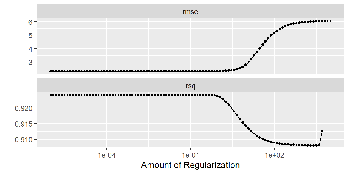
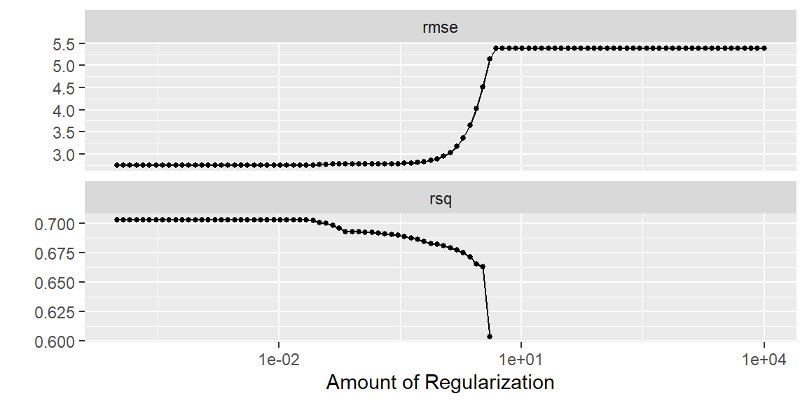
At the point, differing values of penalty has been tried as determined by grid_regular. We can view the results in a few ways. We can plot the mean metric for each value of the penalty, or we can just ask R to show the top few penalties based on either “rmse” or “rsq”.
#plot the metrics for different values of the penaltytune_model |>autoplot()
#find the best penalty in terms of rmsetune_model |>show_best(metric ="rmse")
# A tibble: 5 × 7
     penalty .metric .estimator  mean     n std_err .config
       <dbl> <chr>   <chr>      <dbl> <int>   <dbl> <chr>
1 0.000001   rmse    standard    2.30     5   0.283 Preprocessor1_Model001
2 0.00000126 rmse    standard    2.30     5   0.283 Preprocessor1_Model002
3 0.00000159 rmse    standard    2.30     5   0.283 Preprocessor1_Model003
4 0.00000201 rmse    standard    2.30     5   0.283 Preprocessor1_Model004
5 0.00000254 rmse    standard    2.30     5   0.283 Preprocessor1_Model005
#find the best penalty in terms of rsqtune_model |>show_best(metric ="rsq")
# A tibble: 5 × 7
     penalty .metric .estimator  mean     n std_err .config
       <dbl> <chr>   <chr>      <dbl> <int>   <dbl> <chr>
1 0.572      rsq     standard   0.924     5  0.0139 Preprocessor1_Model058
2 0.000001   rsq     standard   0.924     5  0.0137 Preprocessor1_Model001
3 0.00000126 rsq     standard   0.924     5  0.0137 Preprocessor1_Model002
4 0.00000159 rsq     standard   0.924     5  0.0137 Preprocessor1_Model003
5 0.00000201 rsq     standard   0.924     5  0.0137 Preprocessor1_Model004
Note the “best” penalty value differs from “rmse” to “rsq”. Looking at the plot above, we can see there is not much difference in either metric for the “best” penalty value for either case.
Let’s now get the best penalty from one of the metrics. We will use “rsq” here.
In ridge regression, the estimates shrink to zero for predictors that do not have a significant linear relationship on \(Y\) given the other variables.
The coefficient estimates shrink to zero, but do not equal zero.
The lasso (leastabsoluteshrinkage and selectionoperator) is a shrinkage method like ridge, with subtle but important differences.
The lasso estimate is defined by \[
\begin{align}
Q_{lasso} & =\sum_{i=1}^{n}\left(Y_{i}-\left(\beta_{0}+\beta_{1}X_{1i}+\cdots+\beta_{p-1}X_{p-1,i}\right)\right)^{2}+\lambda\sum_{j=1}^{p-1}\left|\beta_{j}\right|
\end{align}
\tag{19.2}\]
Similarly to ridge regression, the value of \(\lambda\) determines how biased the estimates will be.
As \(\lambda\) increases, the beta coefficients shrink toward zero with the least associated beta coefficients decreasing all the way to 0 before the more strongly associated beta coefficients.
As a result, numerous beta coefficients that are not strongly associated with the outcome are decreased to zero, which is equivalent to removing those variables from the model.
In this way, the lasso can be used as a variableselection method.
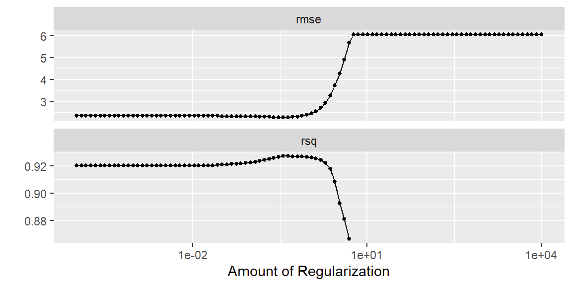
Example 19.3 (Lasso for mtcars) The procedure to fit the lasso is very similar to ridge regression. The only change is in the mixture argument in linear_reg. We will set this to 1 to do lasso.
set.seed(1004) #to reproduce results#prepare the recipedat_recipe =recipe(mpg ~ disp + hp + drat + wt + qsec, data = mtcars) |>step_mutate(log_disp =log(disp),log_hp =log(hp),log_wt =log(wt) ) |>step_rm(disp, hp, wt) |>step_normalize(all_numeric_predictors())#setup the folded data, let's try 5 foldscv_folds =vfold_cv(mtcars, v =5)#setup the model and set penalty to tunelm_model =linear_reg(mixture =1, penalty =tune()) |>set_engine("glmnet")wf =workflow() |>add_recipe(dat_recipe) |>add_model(lm_model)#setup possible values of penalty#this will try 100 different values of penaltypenalty_grid =grid_regular(penalty(range=c(-4, 4)), levels =100)#now tune the grid with everything we just set uptune_model =tune_grid( wf,resamples = cv_folds, grid = penalty_grid,metrics =metric_set(rmse, rsq))tune_model |>autoplot()
We see in this dataset, drat and qsec shrunk to 0. This indicates that they are not important to modeling mpg. The largest magnitude is log_wt which indicates that it has the largest impact on mpg
In the next example, we will fit a lasso model to the bodyfat data.
Example 19.4 (Lasso for the bodyfat data.)
dat =read_table("bodyfat.txt")#prepare the recipedat_recipe =recipe(bfat ~ tri + thigh + midarm, data = dat) |>step_normalize(all_numeric_predictors())#setup the folded data, let's try 5 foldscv_folds =vfold_cv(dat, v =5)#setup the model and set penalty to tunelm_model =linear_reg(mixture =1, penalty =tune()) |>set_engine("glmnet")wf =workflow() |>add_recipe(dat_recipe) |>add_model(lm_model)#setup possible values of penalty#this will try 100 different values of penaltypenalty_grid =grid_regular(penalty(range=c(-4, 4)), levels =100)#now tune the grid with everything we just set uptune_model =tune_grid( wf,resamples = cv_folds, grid = penalty_grid,metrics =metric_set(rmse, rsq))tune_model |>autoplot()
# A tibble: 4 × 3
  term        estimate penalty
  <chr>          <dbl>   <dbl>
1 (Intercept)    20.2   0.0221
2 tri             4.98  0.0221
3 thigh           0     0.0221
4 midarm         -1.53  0.0221
We see that tri has the biggest impact on bfat. The predictor thigh shrunk down to 0. Recall in previous examples when we used the bodyfat data that tri and thigh are highly correlated.
When two predictor variables are highly correlated, the lasso will arbitrarily have one of those variables shrink to zero. The practitioner should understand that the one variable that was not selected could in fact be more appropriate for their model than the one that was selected.